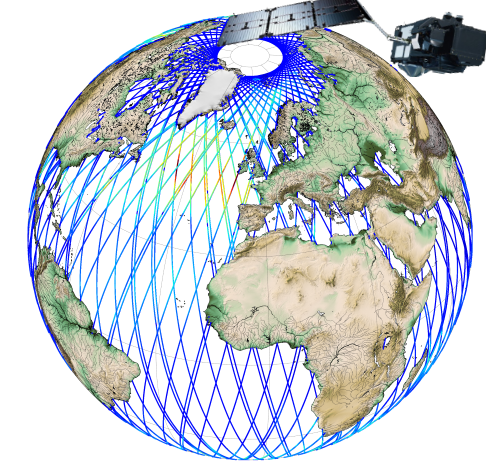
Hauteurs significatives de vagues (SWH) et vitesse du vent, mesurées le long de la trace par les satellites altimétriques CFOSAT (nadir), Sentinel-3A et Sentinel-3B, Jason-3, Saral-AltiKa, Cryosat-2 et HY-2B, en temps quasi-réel (NRT), sur une couverture globale (-66°S/66+N pour Jason-3, -80°S/80°N pour Sentinel-3A et Saral/AltiKa). Un fichier contenant les SWH valides est produit pour chaque mission et pour une fenêtre de temps de 3 heures. Il contient les SWH filtrées (VAVH), les SWH non filtrées (VAVH_UNFILTERED) et la vitesse du vent (wind_speed). Les mesures de hauteurs de vagues sont calculées à partir du front de montée de la forme d'onde altimétrique. Pour Sentinel-3A et 3B, elles sont déduites de l'altimètre SAR.

'''This product has been archived''' '''DEFINITION''' The temporal evolution of thermosteric sea level in an ocean layer is obtained from an integration of temperature driven ocean density variations, which are subtracted from a reference climatology to obtain the fluctuations from an average field. The regional thermosteric sea level values are then averaged from 60°S-60°N aiming to monitor interannual to long term global sea level variations caused by temperature driven ocean volume changes through thermal expansion as expressed in meters (m). '''CONTEXT''' The global mean sea level is reflecting changes in the Earth’s climate system in response to natural and anthropogenic forcing factors such as ocean warming, land ice mass loss and changes in water storage in continental river basins. Thermosteric sea-level variations result from temperature related density changes in sea water associated with volume expansion and contraction. Global thermosteric sea level rise caused by ocean warming is known as one of the major drivers of contemporary global mean sea level rise (Cazenave et al., 2018; Oppenheimer et al., 2019). '''CMEMS KEY FINDINGS''' Since the year 2005 the upper (0-2000m) near-global (60°S-60°N) thermosteric sea level rises at a rate of 1.3±0.2 mm/year. Note: The key findings will be updated annually in November, in line with OMI evolutions. '''DOI (product):''' https://doi.org/10.48670/moi-00240

'''Short description:''' Multi-Year mono-mission satellite-based integral parameters derived from the directional wave spectra. Using linear propagation wave model, only wave observations that can be back-propagated to wave converging regions are considered. The dataset parameters includes partition significant wave height, partition peak period and partition peak or principal direction given along swell propagation path in space and time at a 3-hour timestep, from source to land. Validity flags are also included for each parameter and indicates the valid time steps along propagation (eg. no propagation for significant wave height close to the storm source or any integral parameter when reaching the land). The integral parameters at observation point are also available together with a quality flag based on the consistency between each propagated observation and the overall swell field.This product is processed by the WAVE-TAC multi-mission SAR data processing system. It processes data from the following SAR missions: Sentinel-1A and Sentinel-1B.One file is produced for each mission and is available in two formats: one gathering in one netcdf file all observations related to the same swell field, and for another all observations available in a 3-hour time range, and for both formats, propagated information from source to land. '''DOI (product) :''' https://doi.org/10.48670/moi-00174

'''Short description:''' Global sea ice thickness from merged L-Band radiometer (SMOS ) and radar altimeter (CryoSat-2, Sentinel-3A/B) observations during freezing season between October and April in the northern hemisphere and April to October in the southern hemisphere. The SMOS mission provides L-band observations and the ice thickness-dependency of brightness temperature enables to estimate the sea-ice thickness for thin ice regimes. Radar altimeters measure the height of the ice surface above the water level, which can be converted into sea ice thickness assuming hydrostatic equilibrium. '''DOI (product) :''' https://doi.org/10.48670/moi-00125

'''DEFINITION''' Heat transport across lines are obtained by integrating the heat fluxes along some selected sections and from top to bottom of the ocean. The values are computed from models’ daily output. The mean value over a reference period (1993-2014) and over the last full year are provided for the ensemble product and the individual reanalysis, as well as the standard deviation for the ensemble product over the reference period (1993-2014). The values are given in PetaWatt (PW). '''CONTEXT''' The ocean transports heat and mass by vertical overturning and horizontal circulation, and is one of the fundamental dynamic components of the Earth’s energy budget (IPCC, 2013). There are spatial asymmetries in the energy budget resulting from the Earth’s orientation to the sun and the meridional variation in absorbed radiation which support a transfer of energy from the tropics towards the poles. However, there are spatial variations in the loss of heat by the ocean through sensible and latent heat fluxes, as well as differences in ocean basin geometry and current systems. These complexities support a pattern of oceanic heat transport that is not strictly from lower to high latitudes. Moreover, it is not stationary and we are only beginning to unravel its variability. '''CMEMS KEY FINDINGS''' The mean transports estimated by the ensemble global reanalysis are comparable to estimates based on observations; the uncertainties on these integrated quantities are still large in all the available products. Note: The key findings will be updated annually in November, in line with OMI evolutions. '''DOI (product):''' https://doi.org/10.48670/moi-00245

'''Short description:''' The Reprocessed (REP) Mediterranean (MED) dataset provides a stable and consistent long-term Sea Surface Temperature (SST) time series over the Mediterranean Sea (and the adjacent North Atlantic box) developed for climate applications. This product consists of daily (nighttime), merged multi-sensor (L3S), satellite-based estimates of the foundation SST (namely, the temperature free, or nearly-free, of any diurnal cycle) at 0.05° resolution grid covering the period from 1st January 1981 to present (approximately one month before real time). The MED-REP-L3S product is built from a consistent reprocessing of the collated level-3 (merged single-sensor, L3C) climate data record (CDR) v.3.0, provided by the ESA Climate Change Initiative (CCI) and covering the period up to 2021, and its interim extension (ICDR) that allows the regular temporal extension for 2022 onwards. '''DOI (product) :''' https://doi.org/10.48670/moi-00314

'''Short description: ''' For the '''Global''' Ocean '''Satellite Observations''', ACRI-ST company (Sophia Antipolis, France) is providing '''Bio-Geo-Chemical (BGC)''' products based on the '''Copernicus-GlobColour''' processor. * Upstreams: SeaWiFS, MODIS, MERIS, VIIRS-SNPP & JPSS1, OLCI-S3A & S3B for the '''multi''' products, and S3A & S3B only for the '''olci''' products. * Variables: Chlorophyll-a ('''CHL'''), Gradient of Chlorophyll-a ('''CHL_gradient'''), Phytoplankton Functional types and sizes ('''PFT'''), Suspended Matter ('''SPM'''), Secchi Transparency Depth ('''ZSD'''), Diffuse Attenuation ('''KD490'''), Particulate Backscattering ('''BBP'''), Absorption Coef. ('''CDM''') and Reflectance ('''RRS'''). * Temporal resolutions: '''daily''' * Spatial resolutions: '''4 km''' and a finer resolution based on olci '''300 meters''' inputs. * Recent products are organized in datasets called Near Real Time ('''NRT''') and long time-series (from 1997) in datasets called Multi-Years ('''MY'''). To find the '''Copernicus-GlobColour''' products in the catalogue, use the search keyword '''GlobColour'''. '''DOI (product) :''' https://doi.org/10.48670/moi-00278

'''Short description:''' Near-Real-Time multi-mission global satellite-based spectral integral parameters. Only valid data are used, based on the L3 corresponding products. Included wave parameters are partition significant wave height, partition peak period and partition peak or principal direction. Those parameters are propagated in space and time at a 3-hour timestep and on a regular space grid, providing information of the swell propagation characteristics, from source to land. The ouput products corresponds to one file per month gathering all the swell systems at a global scale. This product is processed by the WAVE-TAC multi-mission SAR and CFOSAT/SWIM data processing system to serve in near-real time the main operational oceanography and climate forecasting centers in Europe and worldwide. It processes data from the following missions: SAR (Sentinel-1A and Sentinel-1B) and CFOSAT/SWIM. All the spectral parameter measurements are optimally interpolated using swell observations belonging to the same swell field. The spectral data processing system produces wave integral parameters by partition (partition significant wave height, partition peak period and partition peak or principal direction) and the associated standard deviation and density of propagated observations. '''DOI (product) :''' https://doi.org/10.48670/moi-00175

'''DEFINITION''' Ocean heat content (OHC) is defined here as the deviation from a reference period (1993-2014) and is closely proportional to the average temperature change from z1 = 0 m to z2 = 700 m depth: OHC=∫_(z_1)^(z_2)ρ_0 c_p (T_yr-T_clim )dz [1] with a reference density of = 1030 kgm-3 and a specific heat capacity of cp = 3980 J kg-1 °C-1 (e.g. von Schuckmann et al., 2009). Time series of annual mean values area averaged ocean heat content is provided for the Mediterranean Sea (30°N, 46°N; 6°W, 36°E) and is evaluated for topography deeper than 300m. '''CONTEXT''' Knowing how much and where heat energy is stored and released in the ocean is essential for understanding the contemporary Earth system state, variability and change, as the oceans shape our perspectives for the future. The quality evaluation of MEDSEA_OMI_OHC_area_averaged_anomalies is based on the “multi-product” approach as introduced in the second issue of the Ocean State Report (von Schuckmann et al., 2018), and following the MyOcean’s experience (Masina et al., 2017). Six global products and a regional (Mediterranean Sea) product have been used to build an ensemble mean, and its associated ensemble spread. The reference products are: • The Mediterranean Sea Reanalysis at 1/24 degree horizontal resolution (MEDSEA_MULTIYEAR_PHY_006_004, DOI: https://doi.org/10.25423/CMCC/MEDSEA_MULTIYEAR_PHY_006_004_E3R1, Escudier et al., 2020) • Four global reanalyses at 1/4 degree horizontal resolution (GLOBAL_MULTIYEAR_PHY_ENS_001_031): GLORYS, C-GLORS, ORAS5, FOAM • Two observation based products: CORA (INSITU_GLO_PHY_TS_OA_MY_013_052) and ARMOR3D (MULTIOBS_GLO_PHY_TSUV_3D_MYNRT_015_012). Details on the products are delivered in the PUM and QUID of this OMI. '''CMEMS KEY FINDINGS''' The ensemble mean ocean heat content anomaly time series over the Mediterranean Sea shows a continuous increase in the period 1993-2022 at rate of 1.38±0.08 W/m2 in the upper 700m. After 2005 the rate has clearly increased with respect the previous decade, in agreement with Iona et al. (2018). '''DOI (product):''' https://doi.org/10.48670/moi-00261

'''DEFINITION''' Estimates of Ocean Heat Content (OHC) are obtained from integrated differences of the measured temperature and a climatology along a vertical profile in the ocean (von Schuckmann et al., 2018). The products used include three global reanalyses: GLORYS, C-GLORS, ORAS5 (GLOBAL_MULTIYEAR_PHY_ENS_001_031) and two in situ based reprocessed products: CORA5.2 (INSITU_GLO_PHY_TS_OA_MY_013_052) , ARMOR-3D (MULTIOBS_GLO_PHY_TSUV_3D_MYNRT_015_012). Additionally, the time series based on the method of von Schuckmann and Le Traon (2011) has been added. The regional OHC values are then averaged from 60°S-60°N aiming i) to obtain the mean OHC as expressed in Joules per meter square (J/m2) to monitor the large-scale variability and change. ii) to monitor the amount of energy in the form of heat stored in the ocean (i.e. the change of OHC in time), expressed in Watt per square meter (W/m2). Ocean heat content is one of the six Global Climate Indicators recommended by the World Meterological Organisation for Sustainable Development Goal 13 implementation (WMO, 2017). '''CONTEXT''' Knowing how much and where heat energy is stored and released in the ocean is essential for understanding the contemporary Earth system state, variability and change, as the ocean shapes our perspectives for the future (von Schuckmann et al., 2020). Variations in OHC can induce changes in ocean stratification, currents, sea ice and ice shelfs (IPCC, 2019; 2021); they set time scales and dominate Earth system adjustments to climate variability and change (Hansen et al., 2011); they are a key player in ocean-atmosphere interactions and sea level change (WCRP, 2018) and they can impact marine ecosystems and human livelihoods (IPCC, 2019). '''CMEMS KEY FINDINGS''' Since the year 2005, the upper (0-2000m) near-global (60°S-60°N) ocean warms at a rate of 0.9 ± 0.1 W/m2. Note: The key findings will be updated annually in November, in line with OMI evolutions. '''DOI (product):''' https://doi.org/10.48670/moi-00235