DNA sequencing of Crassostrea gigas Pacific oyster spat experimentally infected with OsHV-1 virus from oyster basin of Marennes-Oleron

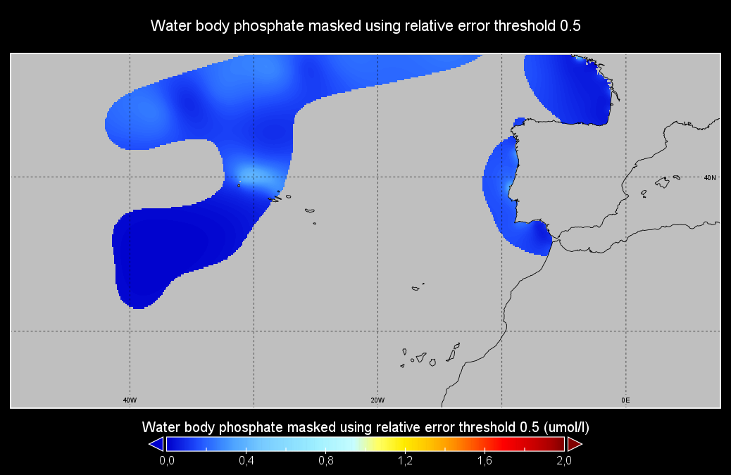
Moving 6-year analysis of Water body phosphate in the NorthEast Atlantic for each season: - winter: January-March, - spring: April-June, - summer: July-September, - autumn: October-December. Every year of the time dimension corresponds to the 6-year centred average of each season. 6-year periods span from 1950/1955 until 2016/2021. Observation data span from 1950 to 2021. Depth levels (IODE standard depths): [0.0, 5.0, 10.0, 20.0, 30.0, 40.0, 50.0, 75.0, 100.0, 125.0, 150.0, 200.0, 250.0, 300.0, 400.0, 500.0, 600.0, 700.0, 800.0, 900.0, 1000.0, 1100.0, 1200.0, 1300.0, 1400.0, 1500.0, 1750.0, 2000.0]. Data sources: observational data from SeaDataNet/EMODNet Chemistry Data Network. Descrption of DIVAnd analysis: the computation was done with DIVAnd (Data-Interpolating Variational Analysis in n dimensions), version 2.7.4, using GEBCO 30 sec topography for the spatial connectivity of water masses. The horizontal resolution of the produced DIVAnd maps is 0.1 degrees. Horizontal correlation length varies from 250km in open sea regions to 50km at the coast. Vertical correlation length is defined as twice the vertical resolution. Signal-to-noise ratio was fixed to 1 for vertical profiles and 0.1 for time series to account for the redundancy in the time series observations. A logarithmic transformation (DIVAnd.Anam.loglin) was applied to the data prior to the analysis to avoid unrealistic negative values. Background field: a vertically-filtered profile of the seasonal data mean value (including all years) is substracted from the data. Detrending of data: no, advection constraint applied: no. Units: umol/l.

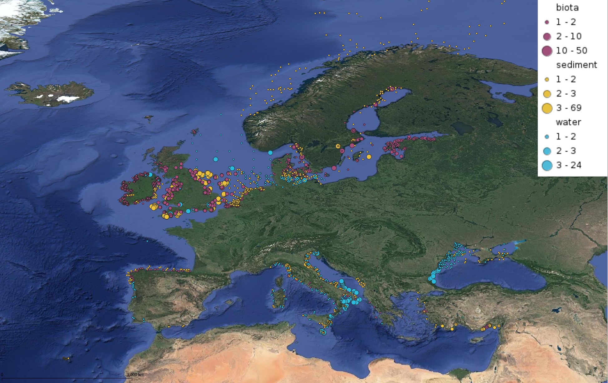
This product displays for Hexachlorobenzene, positions with values counts that have been measured per matrix for each year and are present in EMODnet regional contaminants aggregated datasets, v2022. The product displays positions for every available year.

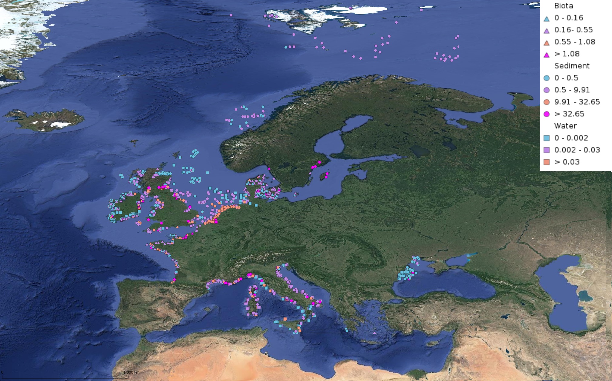
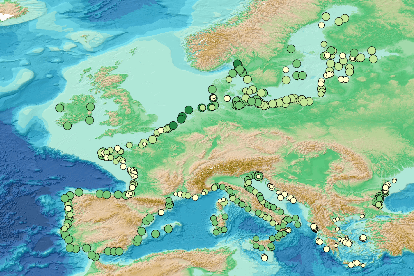
This product displays for Anthracene, median values of the last 6 available years that have been measured per matrix and are present in EMODnet regional contaminants aggregated datasets, v2022. The median values ranges are derived from the following percentiles: 0-25%, 25-75%, 75-90%, >90%. Only "good data" are used, namely data with Quality Flag=1, 2, 6, Q (SeaDataNet Quality Flag schema). For water, only surface values are used (0-15 m), for sediment and biota data at all depths are used.

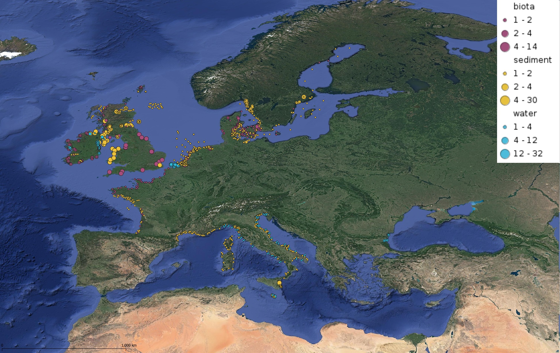
This product displays for Tributyltin, positions with values counts that have been measured per matrix for each year and are present in EMODnet regional contaminants aggregated datasets, v2022. The product displays positions for every available year.

This visualization product displays the number of Marine Strategy Framework Directive (MSFD) monitoring surveys and the associated temporal coverage per beach. EMODnet Chemistry included the collection of marine litter in its 3rd phase. Since the beginning of 2018, data of beach litter have been gathered and processed in the EMODnet Chemistry Marine Litter Database (MLDB). The harmonization of all the data has been the most challenging task considering the heterogeneity of the data sources, sampling protocols and reference lists used on a European scale. Preliminary processing were necessary to harmonize all the data: - Exclusion of OSPAR 1000 protocol: in order to follow the approach of OSPAR that it is not including these data anymore in the monitoring; - Selection of MSFD surveys only (exclusion of other monitoring, cleaning and research operations); - Exclusion of beaches without coordinates. More information is available in the attached documents. Warning: the absence of data on the map doesn't necessarily mean that they don't exist, but that no information has been entered in the Marine Litter Database for this area.

This dataset comprises the global frequency, classification and distribution of marine heat waves (MHWs) from 1996-2020, in Chauhan et al. 2023 (https://doi.org/10.3389/fmars.2023.1177571). The classification was done based on their attributes and using different baselines. Daily SST values were extracted from the NOAA-OISST v2 high-resolution (0.25°) dataset from 1982-2020. MHWs were detected using the method presented by Hobday et al. 2016 (https://doi.org/10.1016/j.pocean.2015.12.014), and by using the 95th percentile of the accumulated temperature distribution to flag the extreme events. A shifting baseline of 8-year rolling period was selected between the years 1982-1996, since this period shows relatively stable maximum values of temperature across different ocean regions. The shifting baseline aims to account for the decadal changes of westerly winds, temperatures and ocean gyres circulations. The classification was done using the KMeans clustering algorithm to identify the relevant features of MHWs and classify them into separate groups based on feature similarities. This algorithm takes MHW features, namely duration, maximum intensity, rate onset and rate decline, as input vectors and applies clustering in the 4-dimensional feature space where each data point represents an MHW event. Note that all the MHWs features are standardized because unequal variances can put more weight on variables with smaller variances. This record comprehends the geospatial datasets of: Average number of MHW days per year (i.e., the sum of all MHW days divided by the total number of years, 1996-2020). Average cumulative intensity per year (i.e., the sum of cumulative intensity divided by the total number of years, 1996-2020). Total number of MHW events across the different periods averaged on the total number of years (1989-2020). The period 1982-1988 was only used as an initial baseline without calculating MHWs. Spatial distribution of three MHW categories: moderate MHWs, abrupt and Intense MHWs and extreme MHWs; displaying the total number of MHW days normalized by the number of years considered (i.e., 1989-2020). Distribution of Extreme MHWs across the different periods (A) 1989-1996, (B) 1997-2004, (C) 2005-2012, (D) 2013-2020. The relative frequency (γ) is a ratio of extreme MHWs in a specific period and all extreme MHWs in the same cluster for all periods.

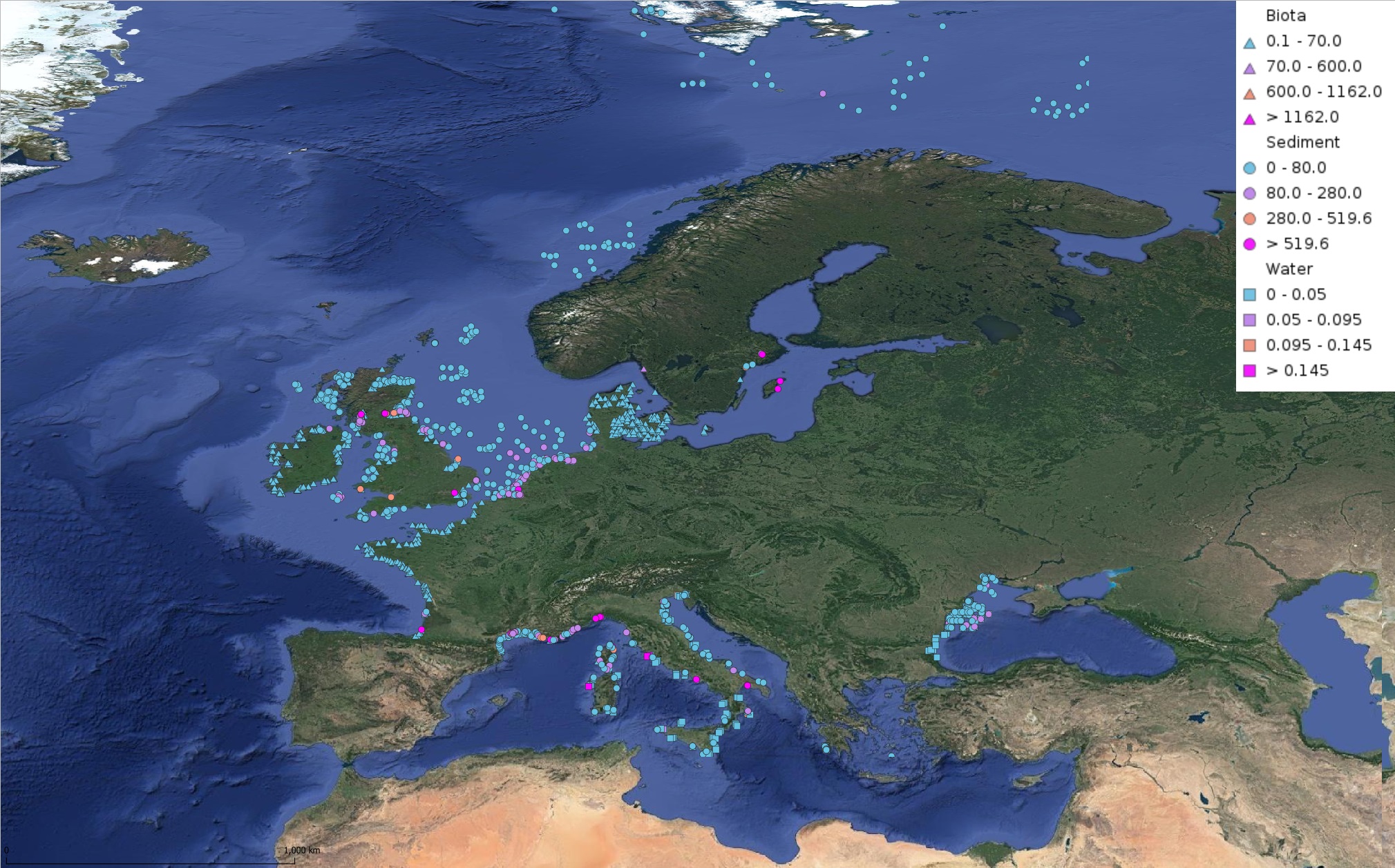
This product displays for Fluoranthene, median values of the last 6 available years that have been measured per matrix and are present in EMODnet regional contaminants aggregated datasets, v2022. The median values ranges are derived from the following percentiles: 0-25%, 25-75%, 75-90%, >90%. Only "good data" are used, namely data with Quality Flag=1, 2, 6, Q (SeaDataNet Quality Flag schema). For water, only surface values are used (0-15 m), for sediment and biota data at all depths are used.

'''DEFINITION''' The OMI_EXTREME_SL_NORTHWESTSHELF_slev_mean_and_anomaly_obs indicator is based on the computation of the 99th and the 1st percentiles from in situ data (observations). It is computed for the variable sea level measured by tide gauges along the coast. The use of percentiles instead of annual maximum and minimum values, makes this extremes study less affected by individual data measurement errors. The annual percentiles referred to annual mean sea level are temporally averaged and their spatial evolution is displayed in the dataset omi_extreme_sl_northwestshelf_slev_mean_and_anomaly_obs, jointly with the anomaly in the target year. This study of extreme variability was first applied to sea level variable (Pérez Gómez et al 2016) and then extended to other essential variables, sea surface temperature and significant wave height (Pérez Gómez et al 2018). '''CONTEXT''' Sea level (SLEV) is one of the Essential Ocean Variables most affected by climate change. Global mean sea level rise has accelerated since the 1990’s (Abram et al., 2019, Legeais et al., 2020), due to the increase of ocean temperature and mass volume caused by land ice melting (WCRP, 2018). Basin scale oceanographic and meteorological features lead to regional variations of this trend that combined with changes in the frequency and intensity of storms could also rise extreme sea levels up to one metre by the end of the century (Vousdoukas et al., 2020, Tebaldi et al., 2021). This will significantly increase coastal vulnerability to storms, with important consequences on the extent of flooding events, coastal erosion and damage to infrastructures caused by waves (Boumis et al., 2023). The increase in extreme sea levels over recent decades is, therefore, primarily due to the rise in mean sea level. Note, however, that the methodology used to compute this OMI removes the annual 50th percentile, thereby discarding the mean sea level trend to isolate changes in storminess. The North West Shelf area presents positive sea level trends with higher trend estimates in the German Bight and around Denmark, and lower trends around the southern part of Great Britain (Dettmering et al., 2021). '''COPERNICUS MARINE SERVICE KEY FINDINGS''' The completeness index criteria is fulfilled by 33 stations in 2023, one less than in 2022 (32). The mean 99th percentiles present a large spatial variability related to the tidal pattern, with largest values found in East England and at the entrance of the English channel, and lowest values along the Danish and Swedish coasts, ranging from the 3.08 m above mean sea level in Immingan (East England) to 0.45 m above mean sea level in Tregde (Norway). The standard deviation of annual 99th percentiles ranges between 2-3 cm in the western part of the region (e.g.: 2 cm in Harwich, 3 cm in Dunkerke) and 7-8 cm in the eastern part and the Kattegat (e.g. 8 cm in Stenungsund, Sweden). The 99th percentile anomalies for 2023 show overall slightly negative values except in the Kattegat (Eastern part), with maximum significant values of +11 cm in Hornbaek (Denmark), and +10 cm in Ringhals (Sweden). '''DOI (product):''' https://doi.org/10.48670/moi-00272

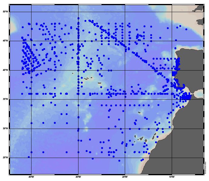
EMODnet Chemistry aims to provide access to marine chemistry datasets and derived data products concerning eutrophication, acidity and contaminants. The importance of the selected substances and other parameters relates to the Marine Strategy Framework Directive (MSFD). This aggregated dataset contains all unrestricted EMODnet Chemistry data on potential hazardous substances, despite the fact that some data might not be related to pollution (e.g. collected by deep corer). Temperature, salinity and additional parameters are included when available. It covers the Northeast Atlantic Ocean (40W). Data were harmonised and validated by the '‘IFREMER / IDM / SISMER - Scientific Information Systems for the SEA’ in France. The dataset contains water (profiles), sediment (profiles and timeseries) and biota (timeseries). The temporal coverage is 1974–2018 for water measurements, 1966–2014 for sediment measurements and 1979–2021 for biota measurements. Regional datasets concerning contaminants are automatically harvested and the resulting collections are harmonised and validated using ODV Software and following a common methodology for all sea regions ( https://doi.org/10.6092/8b52e8d7-dc92-4305-9337-7634a5cae3f4). Parameter names are based on P01 vocabulary, which relates to BODC Parameter Usage Vocabulary and is available at: https://vocab.nerc.ac.uk/search_nvs/P01/. The harmonised dataset can be downloaded as as an ODV spreadsheet, which is composed of a metadata header followed by tab separated values. This spreadsheet can be imported into ODV Software for visualisation (more information can be found at: https://www.seadatanet.org/Software/ODV). In addition, the same dataset is offered also as a txt file in a long/vertical format, in which each P01 measurement is a record line. Additionally, there are a series of columns that split P01 terms into subcomponents (substance, CAS number, matrix...).This transposed format is more adapted to worksheet applications (e.g. LibreOffice Calc).