 Catalogue PIGMA
2019
Type of resources
Available actions
Topics
Keywords
Contact for the resource
Provided by
Years
Formats
Representation types
Update frequencies
status
Service types
Scale
Resolution
-
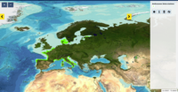
This product displays the stations present in EMODnet validated dataset where fluoranthene levels have been measured in water. EMODnet Chemistry has included the gathering of contaminants data since the beginning of the project in 2009. For the maps for EMODnet Chemistry Phase III, it was requested to plot data per matrix (water,sediment, biota), per biological entity and per chemical substance. The series of relevant map products have been developed according to the criteria D8C1 of the MSFD Directive, specifically focusing on the requirements under the new Commission Decision 2017/848 (17th May 2017). The Commission Decision points to relevant threshold values that are specified in the WFD, as well as relating how these contaminants should be expressed (units and matrix etc.) through the related Directives i.e. Priority substances for Water. EU EQS Directive does not fix any threshold values in sediments. On the contrary Regional Sea Conventions provide some of them, and these values have been taken into account for the development of the visualization products. To produce the maps the following process has been followed: 1. Data collection through SeaDataNet standards (CDI+ODV) 2. Harvesting, harmonization, validation and P01 code decomposition of data 3. SQL query on data sets from point 2 4. Production of map with each point representing at least one record that match the criteria The harmonization of all the data has been the most challenging task considering the heterogeneity of the data sources, sampling protocols. Preliminary processing were necessary to harmonize all the data : • For water: contaminants in the dissolved phase; • For sediment: data on total sediment (regardless of size class) or size class < 2000 μm • For biota: contaminant data will focus on molluscs, on fish (only in the muscle), and on crustaceans • Exclusion of data values equal to 0
-
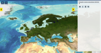
This product displays the stations where mercury has been measured and the values present in EMODnet Chemistry infrastructure are always below the limit of detection or quantification (LOD/LOQ), i.e quality values found in EMODnet validated dataset can be equal to 6 or Q. It is necessary to take into account that LOD/LOQ can change with time. These products aggregate data by station, producing only one final value for each station (above, below or above/below). EMODnet Chemistry has included the gathering of contaminants data since the beginning of the project in 2009. For the maps for EMODnet Chemistry Phase III, it was requested to plot data per matrix (water,sediment, biota), per biological entity and per chemical substance. The series of relevant map products have been developed according to the criteria D8C1 of the MSFD Directive, specifically focusing on the requirements under the new Commission Decision 2017/848 (17th May 2017). The Commission Decision points to relevant threshold values that are specified in the WFD, as well as relating how these contaminants should be expressed (units and matrix etc.) through the related Directives i.e. Priority substances for Water. EU EQS Directive does not fix any threshold values in sediments. On the contrary Regional Sea Conventions provide some of them, and these values have been taken into account for the development of the visualization products. To produce the maps the following process has been followed: 1. Data collection through SeaDataNet standards (CDI+ODV) 2. Harvesting, harmonization, validation and P01 code decomposition of data 3. SQL query on data sets from point 2 4. Production of map with each point representing at least one record that match the criteria The harmonization of all the data has been the most challenging task considering the heterogeneity of the data sources, sampling protocols. Preliminary processing were necessary to harmonize all the data : • For water: contaminants in the dissolved phase; • For sediment: data on total sediment (regardless of size class) or size class < 2000 μm • For biota: contaminant data will focus on molluscs, on fish (only in the muscle), and on crustaceans • Exclusion of data values equal to 0
-
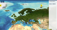
This product displays the stations present in EMODnet validated dataset where naphthalene levels have been measured in water. EMODnet Chemistry has included the gathering of contaminants data since the beginning of the project in 2009. For the maps for EMODnet Chemistry Phase III, it was requested to plot data per matrix (water,sediment, biota), per biological entity and per chemical substance. The series of relevant map products have been developed according to the criteria D8C1 of the MSFD Directive, specifically focusing on the requirements under the new Commission Decision 2017/848 (17th May 2017). The Commission Decision points to relevant threshold values that are specified in the WFD, as well as relating how these contaminants should be expressed (units and matrix etc.) through the related Directives i.e. Priority substances for Water. EU EQS Directive does not fix any threshold values in sediments. On the contrary Regional Sea Conventions provide some of them, and these values have been taken into account for the development of the visualization products. To produce the maps the following process has been followed: 1. Data collection through SeaDataNet standards (CDI+ODV) 2. Harvesting, harmonization, validation and P01 code decomposition of data 3. SQL query on data sets from point 2 4. Production of map with each point representing at least one record that match the criteria The harmonization of all the data has been the most challenging task considering the heterogeneity of the data sources, sampling protocols. Preliminary processing were necessary to harmonize all the data : • For water: contaminants in the dissolved phase; • For sediment: data on total sediment (regardless of size class) or size class < 2000 μm • For biota: contaminant data will focus on molluscs, on fish (only in the muscle), and on crustaceans • Exclusion of data values equal to 0
-
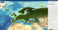
This product displays the stations where fluoranthene has been measured and the values present in EMODnet Chemistry infrastructure are always below the limit of detection or quantification (LOD/LOQ), i.e quality values found in EMODnet validated dataset can be equal to 6 or Q. It is necessary to take into account that LOD/LOQ can change with time. These products aggregate data by station, producing only one final value for each station (above, below or above/below). EMODnet Chemistry has included the gathering of contaminants data since the beginning of the project in 2009. For the maps for EMODnet Chemistry Phase III, it was requested to plot data per matrix (water,sediment, biota), per biological entity and per chemical substance. The series of relevant map products have been developed according to the criteria D8C1 of the MSFD Directive, specifically focusing on the requirements under the new Commission Decision 2017/848 (17th May 2017). The Commission Decision points to relevant threshold values that are specified in the WFD, as well as relating how these contaminants should be expressed (units and matrix etc.) through the related Directives i.e. Priority substances for Water. EU EQS Directive does not fix any threshold values in sediments. On the contrary Regional Sea Conventions provide some of them, and these values have been taken into account for the development of the visualization products. To produce the maps the following process has been followed: 1. Data collection through SeaDataNet standards (CDI+ODV) 2. Harvesting, harmonization, validation and P01 code decomposition of data 3. SQL query on data sets from point 2 4. Production of map with each point representing at least one record that match the criteria The harmonization of all the data has been the most challenging task considering the heterogeneity of the data sources, sampling protocols. Preliminary processing were necessary to harmonize all the data : • For water: contaminants in the dissolved phase; • For sediment: data on total sediment (regardless of size class) or size class < 2000 μm • For biota: contaminant data will focus on molluscs, on fish (only in the muscle), and on crustaceans • Exclusion of data values equal to 0
-
This product displays the stations present in EMODnet validated dataset where naphthalene levels have been measured in biota. EMODnet Chemistry has included the gathering of contaminants data since the beginning of the project in 2009. For the maps for EMODnet Chemistry Phase III, it was requested to plot data per matrix (water,sediment, biota), per biological entity and per chemical substance. The series of relevant map products have been developed according to the criteria D8C1 of the MSFD Directive, specifically focusing on the requirements under the new Commission Decision 2017/848 (17th May 2017). The Commission Decision points to relevant threshold values that are specified in the WFD, as well as relating how these contaminants should be expressed (units and matrix etc.) through the related Directives i.e. Priority substances for Water. EU EQS Directive does not fix any threshold values in sediments. On the contrary Regional Sea Conventions provide some of them, and these values have been taken into account for the development of the visualization products. To produce the maps the following process has been followed: 1. Data collection through SeaDataNet standards (CDI+ODV) 2. Harvesting, harmonization, validation and P01 code decomposition of data 3. SQL query on data sets from point 2 4. Production of map with each point representing at least one record that match the criteria The harmonization of all the data has been the most challenging task considering the heterogeneity of the data sources, sampling protocols. Preliminary processing were necessary to harmonize all the data : • For water: contaminants in the dissolved phase; • For sediment: data on total sediment (regardless of size class) or size class < 2000 μm • For biota: contaminant data will focus on molluscs, on fish (only in the muscle), and on crustaceans • Exclusion of data values equal to 0
-
This product displays the stations where tributyltin has been measured and the values present in EMODnet Chemistry infrastructure are either above or below the limit of detection or quantification (LOD/LOQ), i.e for the substance, in that station, quality values found in EMODnet validated dataset can be equal to 6, Q or 1. It is necessary to take into account that LOD/LOQ can change with time. These products aggregate data by station, producing only one final value for each station (above, below or above/below). EMODnet Chemistry has included the gathering of contaminants data since the beginning of the project in 2009. For the maps for EMODnet Chemistry Phase III, it was requested to plot data per matrix (water,sediment, biota), per biological entity and per chemical substance. The series of relevant map products have been developed according to the criteria D8C1 of the MSFD Directive, specifically focusing on the requirements under the new Commission Decision 2017/848 (17th May 2017). The Commission Decision points to relevant threshold values that are specified in the WFD, as well as relating how these contaminants should be expressed (units and matrix etc.) through the related Directives i.e. Priority substances for Water. EU EQS Directive does not fix any threshold values in sediments. On the contrary Regional Sea Conventions provide some of them, and these values have been taken into account for the development of the visualization products. To produce the maps the following process has been followed: 1. Data collection through SeaDataNet standards (CDI+ODV) 2. Harvesting, harmonization, validation and P01 code decomposition of data 3. SQL query on data sets from point 2 4. Production of map with each point representing at least one record that match the criteria The harmonization of all the data has been the most challenging task considering the heterogeneity of the data sources, sampling protocols. Preliminary processing were necessary to harmonize all the data : • For water: contaminants in the dissolved phase; • For sediment: data on total sediment (regardless of size class) or size class < 2000 μm • For biota: contaminant data will focus on molluscs, on fish (only in the muscle), and on crustaceans • Exclusion of data values equal to 0
-

'''This product has been archived''' For operationnal and online products, please visit https://marine.copernicus.eu '''DEFINITION''' The ocean monitoring indicator of regional mean sea level is derived from the DUACS delayed-time (DT-2021 version) altimeter gridded maps of sea level anomalies based on a stable number of altimeters (two) in the satellite constellation. These products are distributed by the Copernicus Climate Change Service and the Copernicus Marine Service (SEALEVEL_GLO_PHY_CLIMATE_L4_MY_008_057). The mean sea level evolution estimated in the Mediterranean Sea is derived from the average of the gridded sea level maps weighted by the cosine of the latitude. The annual and semi-annual periodic signals are removed (least square fit of sinusoidal function) and the time series is low-pass filtered (175 days cut-off). The curve is corrected for the regional mean effect of the Glacial Isostatic Adjustment (GIA) using the ICE5G-VM2 GIA model (Peltier, 2004). During 1993-1998, the Global men sea level (hereafter GMSL) has been known to be affected by a TOPEX-A instrumental drift (WCRP Global Sea Level Budget Group, 2018; Legeais et al., 2020). This drift led to overestimate the trend of the GMSL during the first 6 years of the altimetry record (about 0.04 mm/y at global scale over the whole altimeter period). A correction of the drift is proposed for the Global mean sea level (Legeais et al., 2020). Whereas this TOPEX-A instrumental drift should also affect the regional mean sea level (hereafter RMSL) trend estimation, this empirical correction is currently not applied to the altimeter sea level dataset and resulting estimated for RMSL. Indeed, the pertinence of the global correction applied at regional scale has not been demonstrated yet and there is no clear consensus achieved on the way to proceed at regional scale. Additionally, the estimate of such a correction at regional scale is not obvious, especially in areas where few accurate independent measurements (e.g. in situ)- necessary for this estimation - are available. The trend uncertainty is provided in a 90% confidence interval (Prandi et al., 2021). This estimate only considers errors related to the altimeter observation system (i.e., orbit determination errors, geophysical correction errors and inter-mission bias correction errors). The presence of the interannual signal can strongly influence the trend estimation considering to the altimeter period considered (Wang et al., 2021; Cazenave et al., 2014). The uncertainty linked to this effect is not taken into account. '''CONTEXT''' The indicator on area averaged sea level is a crucial index of climate change, and individual components contribute to sea level rise, including expansion due to ocean warming and melting of glaciers and ice sheets (WCRP Global Sea Level Budget Group, 2018). According to the recent IPCC 6th assessment report, global mean sea level (GMSL) increased by 0.20 (0.15 to 0.25) m over the period 1901 to 2018 with a rate 25 of rise that has accelerated since the 1960s to 3.7 (3.2 to 4.2) mm yr-1 for the period 2006–2018. Human activity was very likely the main driver of observed GMSL rise since 1970 (IPCC WGII, 2021). The weight of the different contributions evolves with time and in the recent decades the mass change has increased, contributing to the on-going acceleration of the GMSL trend (IPCC, 2022a; Legeais et al., 2020; Horwath et al., 2022). At regional scale, sea level does not change homogenously, and RMSL rise can also be influenced by various other processes, with different spatial and temporal scales, such as local ocean dynamic, atmospheric forcing, Earth gravity and vertical land motion changes (IPCC WGI, 2021). Rising sea level can strongly affect population and infrastructures in coastal areas, increase their vulnerability and risks for food security, particularly in low lying areas and island states. Adverse impacts from floods, storms and tropical cyclones with related losses and damages have increased due to sea level rise, and increase their vulnerability and increase risks for food security, particularly in low lying areas and island states (IPCC, 2022b). Adaptation and mitigation measures such as the restoration of mangroves and coastal wetlands, reduce the risks from sea level rise (IPCC, 2022c). Beside a clear long-term trend, the regional mean sea level variation in the Mediterranean Sea shows an important interannual variability, with a high trend observed before 1999 and lower values afterward. This variability is associated with a variation of the different forcing. Steric effect has been the most important forcing before 1999 (Fenoglio-Marc, 2002; Vigo et al., 2005). Important change of the deep-water formation site also occurred in 1995. The latest is preconditioned by an important change of the sea surface circulation observed in the Ionian Sea in 1997-1998 (e.g. Gačić et al., 2011), under the influence of the North Atlantic Oscillation (NAO) and negative Atlantic Multidecadal Oscillation (AMO) phases (Incarbona et al., 2016). They may also impact the sea level trend in the basin (Vigo et al., 2005). In 2010-2011, high regional mean sea level has been related to enhanced water mass exchange at Gibraltar, under the influence of wind forcing during the negative phase of NAO (Landerer and Volkov, 2013). '''CMEMS KEY FINDINGS''' Over the [1993/01/01, 2021/08/02] period, the basin-wide RMSL in the Mediterranean Sea rises at a rate of 2.7 0.83 mm/year. '''DOI (product):''' https://doi.org/10.48670/moi-00264
-
This product displays the stations present in EMODnet validated dataset where lead levels have been measured in water. EMODnet Chemistry has included the gathering of contaminants data since the beginning of the project in 2009. For the maps for EMODnet Chemistry Phase III, it was requested to plot data per matrix (water,sediment, biota), per biological entity and per chemical substance. The series of relevant map products have been developed according to the criteria D8C1 of the MSFD Directive, specifically focusing on the requirements under the new Commission Decision 2017/848 (17th May 2017). The Commission Decision points to relevant threshold values that are specified in the WFD, as well as relating how these contaminants should be expressed (units and matrix etc.) through the related Directives i.e. Priority substances for Water. EU EQS Directive does not fix any threshold values in sediments. On the contrary Regional Sea Conventions provide some of them, and these values have been taken into account for the development of the visualization products. To produce the maps the following process has been followed: 1. Data collection through SeaDataNet standards (CDI+ODV) 2. Harvesting, harmonization, validation and P01 code decomposition of data 3. SQL query on data sets from point 2 4. Production of map with each point representing at least one record that match the criteria The harmonization of all the data has been the most challenging task considering the heterogeneity of the data sources, sampling protocols. Preliminary processing were necessary to harmonize all the data : • For water: contaminants in the dissolved phase; • For sediment: data on total sediment (regardless of size class) or size class < 2000 μm • For biota: contaminant data will focus on molluscs, on fish (only in the muscle), and on crustaceans • Exclusion of data values equal to 0
-
This product displays the stations present in EMODnet validated dataset where benzo[A]pyrene levels have been measured in biota. EMODnet Chemistry has included the gathering of contaminants data since the beginning of the project in 2009. For the maps for EMODnet Chemistry Phase III, it was requested to plot data per matrix (water,sediment, biota), per biological entity and per chemical substance. The series of relevant map products have been developed according to the criteria D8C1 of the MSFD Directive, specifically focusing on the requirements under the new Commission Decision 2017/848 (17th May 2017). The Commission Decision points to relevant threshold values that are specified in the WFD, as well as relating how these contaminants should be expressed (units and matrix etc.) through the related Directives i.e. Priority substances for Water. EU EQS Directive does not fix any threshold values in sediments. On the contrary Regional Sea Conventions provide some of them, and these values have been taken into account for the development of the visualization products. To produce the maps the following process has been followed: 1. Data collection through SeaDataNet standards (CDI+ODV) 2. Harvesting, harmonization, validation and P01 code decomposition of data 3. SQL query on data sets from point 2 4. Production of map with each point representing at least one record that match the criteria The harmonization of all the data has been the most challenging task considering the heterogeneity of the data sources, sampling protocols. Preliminary processing were necessary to harmonize all the data : • For water: contaminants in the dissolved phase; • For sediment: data on total sediment (regardless of size class) or size class < 2000 μm • For biota: contaminant data will focus on molluscs, on fish (only in the muscle), and on crustaceans • Exclusion of data values equal to 0
-

Zone arrière du point de mutualisation (ZAPM) des territoires gérés par la SPL NATHD déployées