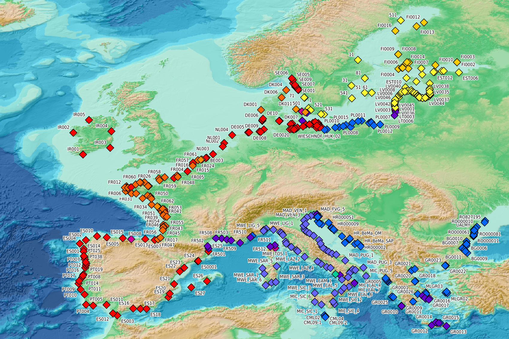
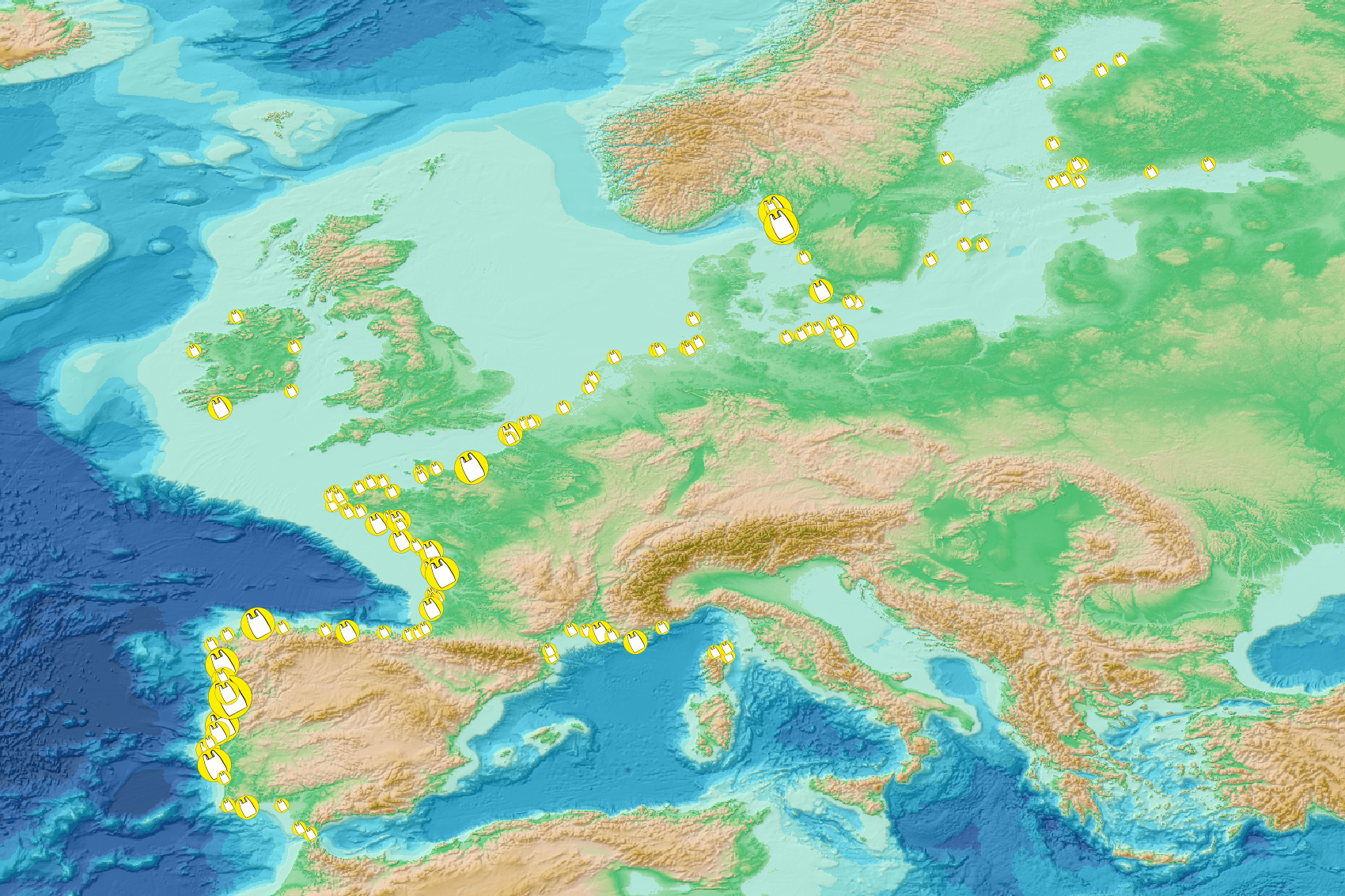
This visualization product displays the cigarette related items abundance of marine macro-litter (> 2.5cm) per beach per year from Marine Strategy Framework Directive (MSFD) monitoring surveys without UNEP-MARLIN data. EMODnet Chemistry included the collection of marine litter in its 3rd phase. Since the beginning of 2018, data of beach litter have been gathered and processed in the EMODnet Chemistry Marine Litter Database (MLDB). The harmonization of all the data has been the most challenging task considering the heterogeneity of the data sources, sampling protocols and reference lists used on a European scale. Preliminary processings were necessary to harmonize all the data: - Exclusion of OSPAR 1000 protocol: in order to follow the approach of OSPAR that it is not including these data anymore in the monitoring; - Selection of MSFD surveys only (exclusion of other monitoring, cleaning and research operations); - Exclusion of beaches without coordinates; - Selection of cigarette related items only. The list of selected items is attached to this metadata. This list was created using EU Marine Beach Litter Baselines, the European Threshold Value for Macro Litter on Coastlines and the Joint list of litter categories for marine macro-litter monitoring from JRC (these three documents are attached to this metadata); - Exclusion of surveys referring to the UNEP-MARLIN list: the UNEP-MARLIN protocol differs from the other types of monitoring in that cigarette butts are surveyed in a 10m square. To avoid comparing abundances from very different protocols, the choice has been made to distinguish in two maps the cigarette related items results associated with the UNEP-MARLIN list from the others; - Normalization of survey lengths to 100m & 1 survey / year: in some case, the survey length was not exactly 100m, so in order to be able to compare the abundance of litter from different beaches a normalization is applied using this formula: Number of cigarette related items of the survey (normalized by 100 m) = Number of cigarette related items of the survey x (100 / survey length) Then, this normalized number of cigarette related items is summed to obtain the total normalized number of cigarette related items for each survey. Finally, the median abundance of cigarette related items for each beach and year is calculated from these normalized abundances of cigarette related items per survey. Sometimes the survey length was null or equal to 0. Assuming that the MSFD protocol has been applied, the length has been set at 100m in these cases. Percentiles 50, 75, 95 & 99 have been calculated taking into account cigarette related items from MSFD monitoring data (excluding UNEP-MARLIN protocol) for all years. More information is available in the attached documents. Warning: the absence of data on the map does not necessarily mean that they do not exist, but that no information has been entered in the Marine Litter Database for this area.

This visualization product displays nets locations where research and monitoring protocols have been applied to collate data on microlitter. Mesh size used with these protocols have been indicated with different colors in the map. EMODnet Chemistry included the collection of marine litter in its 3rd phase. Before 2021, there was no coordinated effort at the regional or European scale for micro-litter. Given this situation, EMODnet Chemistry proposed to adopt the data gathering and data management approach as generally applied for marine data, i.e., populating metadata and data in the CDI Data Discovery and Access service using dedicated SeaDataNet data transport formats. EMODnet Chemistry is currently the official EU collector of micro-litter data from Marine Strategy Framework Directive (MSFD) National Monitoring activities (descriptor 10). A series of specific standard vocabularies or standard terms related to micro-litter have been added to SeaDataNet NVS (NERC Vocabulary Server) Common Vocabularies to describe the micro-litter. European micro-litter data are collected by the National Oceanographic Data Centres (NODCs). Micro-litter map products are generated from NODCs data after a test of the aggregated collection including data and data format checks and data harmonization. A filter is applied to represent only micro-litter sampled according to research and monitoring protocols as MSFD monitoring. Warning: the absence of data on the map does not necessarily mean that they do not exist, but that no information has been entered in the National Oceanographic Data Centre (NODC) for this area.

This visualization product displays the spatial distribution of the sampling effort over the six-years' period 2017-2022. EMODnet Chemistry included the collection of marine litter in its 3rd phase. Since the beginning of 2018, data of seafloor litter collected by international fish-trawl surveys have been gathered and processed in the EMODnet Chemistry Marine Litter Database (MLDB). The harmonization of all the data has been the most challenging task considering the heterogeneity of the data sources, sampling protocols (OSPAR and MEDITS protocols) and reference lists used on a European scale. Moreover, within the same protocol, different gear types are deployed during bottom trawl surveys. The spatial distribution was determined by calculating the number of times each cell was sampled during the period 2017-2022. The corresponding total distance (kms) sampled in each cell is also provided in the attribute table. Information on data processing and calculation are detailed in the attached methodology document. Warning: the absence of data on the map does not necessarily mean that they do not exist, but that no information has been entered in the Marine Litter Database for this area. This work is based on the work presented in the following scientific article: O. Gerigny, M. Brun, M.C. Fabri, C. Tomasino, M. Le Moigne, A. Jadaud, F. Galgani, Seafloor litter from the continental shelf and canyons in French Mediterranean Water: Distribution, typologies and trends, Marine Pollution Bulletin, Volume 146, 2019, Pages 653-666, ISSN 0025-326X, https://doi.org/10.1016/j.marpolbul.2019.07.030.

Rocch, the french "mussel watch", provides chemical data for marine quality management. Once a year, trace metals, organic compounds (chlorinated, PAH, brominated flame retardants, perfluorinated compounds, organotins ...) are analysed in molluscs tissues to check chemical quality according to European Framework Directives and to Regional Seas Convention (OSPAR).

Sardine physiological measurments from september to november 2020

This visualization product displays the type of litter in percent per net per year from research and monitoring protocols. EMODnet Chemistry included the collection of marine litter in its 3rd phase. Before 2021, there was no coordinated effort at the regional or European scale for micro-litter. Given this situation, EMODnet Chemistry proposed to adopt the data gathering and data management approach as generally applied for marine data, i.e., populating metadata and data in the CDI Data Discovery and Access service using dedicated SeaDataNet data transport formats. EMODnet Chemistry is currently the official EU collector of micro-litter data from Marine Strategy Framework Directive (MSFD) National Monitoring activities (descriptor 10). A series of specific standard vocabularies or standard terms related to micro-litter have been added to SeaDataNet NVS (NERC Vocabulary Server) Common Vocabularies to describe the micro-litter. European micro-litter data are collected by the National Oceanographic Data Centres (NODCs). Micro-litter map products are generated from NODCs data after a test of the aggregated collection including data and data format checks and data harmonization. A filter is applied to represent only micro-litter sampled according to research and monitoring protocols as MSFD monitoring. To calculate percentages for each type, formula applied is: Type (%) = (∑number of particles of each type)*100 / (∑number of particles of all type) When the number of micro-litters was not filled or was equal zero, it was not possible to calculate the percentage. Standard vocabularies for micro-litter types are taken from Seadatanet's H01 library (https://vocab.seadatanet.org/v_bodc_vocab_v2/search.asp?lib=H01 ). Some morphological types of micro-litters may have been sampled but were not defined by the protocole applied during the survey. They are represented as « undefined micro-litter items ». Warnings: - the absence of data on the map does not necessarily mean that they do not exist, but that no information has been entered in the National Oceanographic Data Centre (NODC) for this area. - since 03/07/2023, the preferred label « Undefined micro-litter items » has been integrated into the H01 library whereas the labels « microplastic items », « non-plastic man-made micro-particles (e.g. glass, metal, tar) » and «non-plastic filaments (natural fibres, rubber) » have been deprecated. When defined, the material or polymer type can be checked directly in the source data.

The network was initiated by IFREMER from 1993 to 2009 (under the acronym REMORA) to study the rearing performance of the Pacific oyster Crassostrea gigas at a national scale. To do so, the network monitored annually the mortality and growth of standardized batches of 18-month-old oysters. Starting in 1995, the monitoring of the rearing performance of 6-month-old oyster spat was integrated into this network. These sentinel batches were distributed simultaneously each year on 43 sites and were monitored quarterly. These sites were distributed over the main French oyster farming areas and allowed a national coverage of the multiannual evolution of oyster farming performances. Most of the sites were located on the foreshore at comparable levels of immersion. Field studies were carried out by the "Laboratoires Environnement Ressources" (LER) for the sites included in their geographical area of investigation. Following the increase in spat mortality in 2008, the network evolved in 2009 (under the acronym RESCO). From this date, the network selected 13 sites among the 43 sites previously monitored in order to increase the frequency of visits (twice a month) and the number of sentinel batches. More precisely, sentinel batches of oysters corresponding to different origins (wild or hatchery, diploid or triploid) and to two rearing age classes (spat or 18-month-old adults) were selected. The monitoring of environmental variables (temperature, salinity) associated with the 13 sites was also implemented. The actions of the network have thus contributed to disentangle the biotic and abiotic parameters involved in mortality phenomena, taking into account the different compartments (environment / host / infectious agents) likely to interact with the evolution of oyster rearing performance. Finally, since 2015, the network has merged the RESCO and VELYGER networks to adopt the acronym ECOSCOPA. The general objective of this current network is to analyze the causes of spatio-temporal variability of the main life traits (Larval stage - Recruitment - Reproduction - Growth - Survival - Cytogenetic abnormalities) of the cupped oyster in France and to follow their evolution on the long term in the context of climate change. To do this, the network proposes a regular spatio-temporal monitoring of the major proxies of the life cycle of the oyster, organized in three major thematic groups: (1) proxies related to growth, physiological tolerance and survival of experimental sentinel populations over 3 age classes: (2) proxies related to reproduction, larval phase and recruitment of the species throughout its natural range in France, and: (3) proxies related to environmental parameters essential to the species (weather conditions, temperature, salinity, pH, turbidity, chlorophyll a and phytoplankton) at daily or sub-hourly frequencies. Working in a geographical network associating several laboratories, ECOSCOPA provide these monitoring within 8 sites selected among the previous ones to ensure the continuity of the data acquisition. Today, these 8 sites are considered as ecosystems of common interest, contrasted, namely : - The Thau lagoon - The Arcachon basin - The Marennes Oléron basin - The Bourgneuf Bay - The bay of Vilaine - The bay of Brest - The bay of Mont Saint Michel - The bay of Veys The ECOSCOPA network is therefore one of the relevant monitoring tools on a national scale, allowing to objectively measure through different proxies the general state of health of cultivated and wild oyster populations, and this for the different sensitive phases of their life cycle. This network aims at allowing a better evaluation, on the long term, of the biological risks incurred by the sector but also by the ecosystems, in particular under the increasing constraint of climatic and anthropic changes. Figure : Sites monitored by the ECOSCOPA network  

This visualization product displays the fishing & aquaculture related plastic items abundance of marine macro-litter (> 2.5cm) per beach per year from non-MSFD monitoring surveys, research & cleaning operations. EMODnet Chemistry included the collection of marine litter in its 3rd phase. Since the beginning of 2018, data of beach litter have been gathered and processed in the EMODnet Chemistry Marine Litter Database (MLDB). The harmonization of all the data has been the most challenging task considering the heterogeneity of the data sources, sampling protocols and reference lists used on a European scale. Preliminary processings were necessary to harmonize all the data: - Exclusion of OSPAR 1000 protocol: in order to follow the approach of OSPAR that it is not including these data anymore in the monitoring; - Selection of surveys from non-MSFD monitoring, cleaning and research operations; - Exclusion of beaches without coordinates; - Selection of fishing and aquaculture related plastic items only. The list of selected items is attached to this metadata. This list was created using EU Marine Beach Litter Baselines, the European Threshold Value for Macro Litter on Coastlines and the Joint list of litter categories for marine macro-litter monitoring from JRC (these three documents are attached to this metadata). The selection was adapted to the Joint list of litter categories fishing gears identification and therefore contains some differences with the selection made for previously published versions of this product; - Exclusion of surveys without associated length; - Normalization of survey lengths to 100m & 1 survey / year: in some case, the survey length was not 100m, so in order to be able to compare the abundance of litter from different beaches a normalization is applied using this formula: Number of fishing & aquaculture related plastic items of the survey (normalized by 100 m) = Number of fishing & aquaculture related items of the survey x (100 / survey length) Then, this normalized number of fishing & aquaculture related plastic items is summed to obtain the total normalized number of fishing & aquaculture related plastic items for each survey. Finally, the median abundance of fishing & aquaculture related plastic items for each beach and year is calculated from these normalized abundances of fishing & aquaculture related items per survey. Percentiles 50, 75, 95 & 99 have been calculated taking into account fishing & aquaculture related plastic items from other sources data for all years. More information is available in the attached documents. Warning: the absence of data on the map does not necessarily mean that they do not exist, but that no information has been entered in the Marine Litter Database for this area.

'''DEFINITION''' Estimates of Ocean Heat Content (OHC) are obtained from integrated differences of the measured temperature and a climatology along a vertical profile in the ocean (von Schuckmann et al., 2018). The products used include three global reanalyses: GLORYS, C-GLORS, ORAS5 (GLOBAL_MULTIYEAR_PHY_ENS_001_031) and two in situ based reprocessed products: CORA5.2 (INSITU_GLO_PHY_TS_OA_MY_013_052) , ARMOR-3D (MULTIOBS_GLO_PHY_TSUV_3D_MYNRT_015_012). Additionally, the time series based on the method of von Schuckmann and Le Traon (2011) has been added. The regional OHC values are then averaged from 60°S-60°N aiming i) to obtain the mean OHC as expressed in Joules per meter square (J/m2) to monitor the large-scale variability and change. ii) to monitor the amount of energy in the form of heat stored in the ocean (i.e. the change of OHC in time), expressed in Watt per square meter (W/m2). Ocean heat content is one of the six Global Climate Indicators recommended by the World Meterological Organisation for Sustainable Development Goal 13 implementation (WMO, 2017). '''CONTEXT''' Knowing how much and where heat energy is stored and released in the ocean is essential for understanding the contemporary Earth system state, variability and change, as the ocean shapes our perspectives for the future (von Schuckmann et al., 2020). Variations in OHC can induce changes in ocean stratification, currents, sea ice and ice shelfs (IPCC, 2019; 2021); they set time scales and dominate Earth system adjustments to climate variability and change (Hansen et al., 2011); they are a key player in ocean-atmosphere interactions and sea level change (WCRP, 2018) and they can impact marine ecosystems and human livelihoods (IPCC, 2019). '''CMEMS KEY FINDINGS''' Since the year 2005, the near-surface (0-300m) near-global (60°S-60°N) ocean warms at a rate of 0.4 ± 0.1 W/m2. Note: The key findings will be updated annually in November, in line with OMI evolutions. '''DOI (product):''' https://doi.org/10.48670/moi-00233

This visualization product displays the spatial distribution of the sampling effort over the six-years' period 2017-2022 from research and monitoring protocols. EMODnet Chemistry included the collection of marine litter in its 3rd phase. Before 2021, there was no coordinated effort at the regional or European scale for micro-litter. Given this situation, EMODnet Chemistry proposed to adopt the data gathering and data management approach as generally applied for marine data, i.e., populating metadata and data in the CDI Data Discovery and Access service using dedicated SeaDataNet data transport formats. EMODnet Chemistry is currently the official EU collector of micro-litter data from Marine Strategy Framework Directive (MSFD) National Monitoring activities (descriptor 10). A series of specific standard vocabularies or standard terms related to micro-litter have been added to SeaDataNet NVS (NERC Vocabulary Server) Common Vocabularies to describe the micro-litter. European micro-litter data are collected by the National Oceanographic Data Centres (NODCs). Micro-litter map products are generated from NODCs data after a test of the aggregated collection including data and data format checks and data harmonization. A filter is applied to represent only micro-litter samplings carried out according to research and monitoring protocols as MSFD monitoring. The spatial distribution was then determined by calculating the number of times each cell was sampled during the period 2017-2022. The corresponding total distance (kms) sampled in each cell is also provided in the attribute table. Warning: the absence of data on the map does not necessarily mean that they do not exist, but that no information has been entered in the National Oceanographic Data Centre (NODC) for this area.