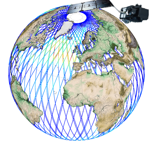
Hauteurs significatives de vagues (SWH) et vitesse du vent, mesurées le long de la trace par les satellites altimétriques CFOSAT (nadir), Sentinel-3A et Sentinel-3B, Jason-3, Saral-AltiKa, Cryosat-2 et HY-2B, en temps quasi-réel (NRT), sur une couverture globale (-66°S/66+N pour Jason-3, -80°S/80°N pour Sentinel-3A et Saral/AltiKa). Un fichier contenant les SWH valides est produit pour chaque mission et pour une fenêtre de temps de 3 heures. Il contient les SWH filtrées (VAVH), les SWH non filtrées (VAVH_UNFILTERED) et la vitesse du vent (wind_speed). Les mesures de hauteurs de vagues sont calculées à partir du front de montée de la forme d'onde altimétrique. Pour Sentinel-3A et 3B, elles sont déduites de l'altimètre SAR.

'''Short description:''' For the Global Ocean- Gridded objective analysis fields of temperature and salinity using profiles from the in-situ near real time database are produced monthly. Objective analysis is based on a statistical estimation method that allows presenting a synthesis and a validation of the dataset, providing a support for localized experience (cruises), providing a validation source for operational models, observing seasonal cycle and inter-annual variability. '''DOI (product) :''' https://doi.org/10.48670/moi-00037

"'Short description: ''' Global Ocean - This delayed mode product designed for reanalysis purposes integrates the best available version of in situ data for ocean surface and subsurface currents. Current data from 5 different types of instruments are distributed: * The drifter's near-surface velocities computed from their position measurements. In addition, a wind slippage correction is provided from 1993. Information on the presence of the drogue of the drifters is also provided. * The near-surface zonal and meridional total velocities, and near-surface radial velocities, measured by High Frequency (HF) radars that are part of the European HF radar Network. These data are delivered together with standard deviation of near-surface zonal and meridional raw velocities, Geometrical Dilution of Precision (GDOP), quality flags and metadata. * The zonal and meridional velocities, at parking depth (mostly around 1000m) and at the surface, calculated along the trajectories of the floats which are part of the Argo Program. * The velocity profiles within the water column coming from Acoustic Doppler Current Profiler (vessel mounted ADCP, Moored ADCP, saildrones) platforms * The near-surface and subsurface velocities calculated from gliders (autonomous underwater vehicle) trajectories '''DOI (product) :''' https://doi.org/10.17882/86236

'''DEFINITION''' The temporal evolution of thermosteric sea level in an ocean layer is obtained from an integration of temperature driven ocean density variations, which are subtracted from a reference climatology to obtain the fluctuations from an average field. The regional thermosteric sea level values are then averaged from 60°S-60°N aiming to monitor interannual to long term global sea level variations caused by temperature driven ocean volume changes through thermal expansion as expressed in meters (m). '''CONTEXT''' Most of the interannual variability and trends in regional sea level is caused by changes in steric sea level. At mid and low latitudes, the steric sea level signal is essentially due to temperature changes, i.e. the thermosteric effect (Stammer et al., 2013, Meyssignac et al., 2016). Salinity changes play only a local role. Regional trends of thermosteric sea level can be significantly larger compared to their globally averaged versions (Storto et al., 2018). Except for shallow shelf sea and high latitudes (> 60° latitude), regional thermosteric sea level variations are mostly related to ocean circulation changes, in particular in the tropics where the sea level variations and trends are the most intense over the last two decades. '''CMEMS KEY FINDINGS''' Significant (i.e. when the signal exceeds the noise) regional trends for the period 2005-2019 from the Copernicus Marine Service multi-ensemble approach show a thermosteric sea level rise at rates ranging from the global mean average up to more than 8 mm/year. There are specific regions where a negative trend is observed above noise at rates up to about -8 mm/year such as in the subpolar North Atlantic, or the western tropical Pacific. These areas are characterized by strong year-to-year variability (Dubois et al., 2018; Capotondi et al., 2020). Note: The key findings will be updated annually in November, in line with OMI evolutions. '''DOI (product):''' https://doi.org/10.48670/moi-00241

'''Short description:''' The High-Resolution Ocean Colour (HR-OC) Consortium (Brockmann Consult, Royal Belgian Institute of Natural Sciences, Flemish Institute for Technological Research) distributes Remote Sensing Reflectances (RRS, expressed in sr-1), Turbidity (TUR, expressed in FNU), Solid Particulate Matter Concentration (SPM, expressed in mg/l), spectral particulate backscattering (BBP, expressed in m-1) and chlorophyll-a concentration (CHL, expressed in µg/l) for the Sentinel 2/MSI sensor at 100m resolution for a 20km coastal zone. The products are delivered on a geographic lat-lon grid (EPSG:4326). To limit file size the products are provided in tiles of 600x800 km². RRS and BBP are delivered at nominal central bands of 443, 492, 560, 665, 704, 740, 783, 865 nm. The primary variable from which it is virtually possible to derive all the geophysical and transparency products is the spectral RRS. This, together with the spectral BBP, constitute the category of the 'optics' products. The spectral BBP product is generated from the RRS products using a quasi-analytical algorithm (Lee et al. 2002). The 'transparency' products include TUR and SPM). They are retrieved through the application of automated switching algorithms to the RRS spectra adapted to varying water conditions (Novoa et al. 2017). The GEOPHYSICAL product consists of the Chlorophyll-a concentration (CHL) retrieved via a multi-algorithm approach with optimized quality flagging (O'Reilly et al. 2019, Gons et al. 2005, Lavigne et al. 2021). The NRT products are generally provided withing 24 hours up to 3 days after end of the day.The RRS product is accompanied by a relative uncertainty estimate (unitless) derived by direct comparison of the products to corresponding fiducial reference measurements provided through the AERONET-OC network. The current day data temporal consistency is evaluated as Quality Index (QI) for TUR, SPM and CHL: QI=(CurrentDataPixel-ClimatologyDataPixel)/STDDataPixel where QI is the difference between current data and the relevant climatological field as a signed multiple of climatological standard deviations (STDDataPixel). '''Processing information:''' The HR-OC processing system is deployed on Creodias where Sentinel 2/MSI L1C data are available. The production control element is being hosted within the infrastructure of Brockmann Consult. The processing chain consists of: * Resampling to 60m and mosaic generation of the set of Sentinel-2 MSI L1C granules of a single overpass that cover a single UTM zone. * Application of a glint correction taking into account the detector viewing angles * Application of a coastal mask with 20km water + 20km land. The result is a L1C mosaic tile with data just in the coastal area optimized for compression. * Level 2 processing with pixel identification (IdePix), atmospheric correction (C2RCC and ACOLITE or iCOR), in-water processing and merging (HR-OC L2W processor). The result is a 60m product with the same extent as the L1C mosaic, with variables for optics, transparency, and geophysics, and with data filled in the water part of the coastal area. * invalid pixel identification takes into account corrupted (L1) pixels, clouds, cloud shadow, glint, dry-fallen intertidal flats, coastal mixed-pixels, sea ice, melting ice, floating vegetation, non-water objects, and bottom reflection. * Daily L3 aggregation merges all Level 2 mosaics of a day intersecting with a target tile. All valid water pixels are included in the 20km coastal stripes; all other values are set to NaN. There may be more than a single overpass a day, in particular in the northern regions. The main contribution usually is the mosaic of the zone, but also adjacent mosaics may overlap. This step comprises resampling to the 100m target grid. * Monthly L4 aggregation combines all Level 3 products of a month and a single tile. The output is a set of 3 NetCDF datasets for optics, transparency, and geophysics respectively, for the tile and month. * Gap filling combines all daily products of a period and generates (partially) gap-filled daily products again. The output of gap filling are 3 datasets for optics (BBP443 only), transparency, and geophysics per day. '''Description of observation methods/instruments:''' Ocean colour technique exploits the emerging electromagnetic radiation from the sea surface in different wavelengths. The spectral variability of this signal defines the so-called ocean colour which is affected by the presence of phytoplankton. '''Quality / Accuracy / Calibration information:''' A detailed description of the calibration and validation activities performed over this product can be found on the CMEMS web portal and in CMEMS-BGP_HR-QUID-009-201to212. '''Suitability, Expected type of users / uses:''' This product is meant for use for educational purposes and for the managing of the marine safety, marine resources, marine and coastal environment and for climate and seasonal studies. '''Dataset names: ''' *cmems_obs_oc_ibi_bgc_geophy_nrt_l3-hr_P1D-v01 *cmems_obs_oc_ibi_bgc_transp_nrt_l3-hr_P1D-v01 *cmems_obs_oc_ibi_bgc_optics_nrt_l3-hr_P1D-v01 '''Files format:''' *netCDF-4, CF-1.7 *INSPIRE compliant. '''DOI (product) :''' https://doi.org/10.48670/moi-00109

'''Short description: ''' For the '''Global''' Ocean '''Satellite Observations''', ACRI-ST company (Sophia Antipolis, France) is providing '''Bio-Geo-Chemical (BGC)''' products based on the '''Copernicus-GlobColour''' processor. * Upstreams: SeaWiFS, MODIS, MERIS, VIIRS-SNPP & JPSS1, OLCI-S3A & S3B for the '''""multi""''' products, and S3A & S3B only for the '''""olci""''' products. * Variables: Chlorophyll-a ('''CHL'''), Gradient of Chlorophyll-a ('''CHL_gradient'''), Phytoplankton Functional types and sizes ('''PFT'''), Suspended Matter ('''SPM'''), Secchi Transparency Depth ('''ZSD'''), Diffuse Attenuation ('''KD490'''), Particulate Backscattering ('''BBP'''), Absorption Coef. ('''CDM''') and Reflectance ('''RRS'''). * Temporal resolutions: '''daily'''. * Spatial resolutions: '''1 km''' and a finer resolution based on olci '''300 meters''' inputs. * Recent products are organized in datasets called Near Real Time ('''NRT''') and long time-series (from 1997) in datasets called Multi-Years ('''MY'''). To find the '''Copernicus-GlobColour''' products in the catalogue, use the search keyword '''""GlobColour""'''. '''DOI (product) :''' https://doi.org/10.48670/moi-00286

'''DEFINITION''' Estimates of Ocean Heat Content (OHC) are obtained from integrated differences of the measured temperature and a climatology along a vertical profile in the ocean (von Schuckmann et al., 2018). The regional OHC values are then averaged from 60°S-60°N aiming i) to obtain the mean OHC as expressed in Joules per meter square (J/m2) to monitor the large-scale variability and change. ii) to monitor the amount of energy in the form of heat stored in the ocean (i.e. the change of OHC in time), expressed in Watt per square meter (W/m2). Ocean heat content is one of the six Global Climate Indicators recommended by the World Meterological Organisation for Sustainable Development Goal 13 implementation (WMO, 2017). '''CONTEXT''' Knowing how much and where heat energy is stored and released in the ocean is essential for understanding the contemporary Earth system state, variability and change, as the ocean shapes our perspectives for the future (von Schuckmann et al., 2020). Variations in OHC can induce changes in ocean stratification, currents, sea ice and ice shelfs (IPCC, 2019; 2021); they set time scales and dominate Earth system adjustments to climate variability and change (Hansen et al., 2011); they are a key player in ocean-atmosphere interactions and sea level change (WCRP, 2018) and they can impact marine ecosystems and human livelihoods (IPCC, 2019). '''CMEMS KEY FINDINGS''' Since the year 2005, the upper (0-2000m) near-global (60°S-60°N) ocean warms at a rate of 1.0 ± 0.1 W/m2. Note: The key findings will be updated annually in November, in line with OMI evolutions. '''DOI (product):''' https://doi.org/10.48670/moi-00235

'''Short description:''' For the Baltic Sea- The DMI Sea Surface Temperature L3S aims at providing daily multi-sensor supercollated data at 0.03deg. x 0.03deg. horizontal resolution, using satellite data from infra-red radiometers. Uses SST satellite products from these sensors: NOAA AVHRRs 7, 9, 11, 14, 16, 17, 18 , Envisat ATSR1, ATSR2 and AATSR. '''DOI (product) :''' https://doi.org/10.48670/moi-00154

'''DEFINITION''' The indicator of the Kuroshio extension phase variations is based on the standardized high frequency altimeter Eddy Kinetic Energy (EKE) averaged in the area 142-149°E and 32-37°N and computed from the DUACS (https://duacs.cls.fr) delayed-time (reprocessed version DT-2021, CMEMS SEALEVEL_GLO_PHY_L4_MY_008_047, including “my” (multi-year) & “myint” (multi-year interim) datasets) and near real-time (CMEMS SEALEVEL_GLO_PHY_L4_NRT _008_046) altimeter sea level gridded products. The change in the reprocessed version (previously DT-2018) and the extension of the mean value of the EKE (now 27 years, previously 20 years) induce some slight changes not impacting the general variability of the Kuroshio extension (correlation coefficient of 0.988 for the total period, 0.994 for the delayed time period only). ""CONTEXT"" The Kuroshio Extension is an eastward-flowing current in the subtropical western North Pacific after the Kuroshio separates from the coast of Japan at 35°N, 140°E. Being the extension of a wind-driven western boundary current, the Kuroshio Extension is characterized by a strong variability and is rich in large-amplitude meanders and energetic eddies (Niiler et al., 2003; Qiu, 2003, 2002). The Kuroshio Extension region has the largest sea surface height variability on sub-annual and decadal time scales in the extratropical North Pacific Ocean (Jayne et al., 2009; Qiu and Chen, 2010, 2005). Prediction and monitoring of the path of the Kuroshio are of huge importance for local economies as the position of the Kuroshio extension strongly determines the regions where phytoplankton and hence fish are located. Unstable (contracted) phase of the Kuroshio enhance the production of Chlorophyll (Lin et al., 2014). ""CMEMS KEY FINDINGS"" The different states of the Kuroshio extension phase have been presented and validated by (Bessières et al., 2013) and further reported by Drévillon et al. (2018) in the Copernicus Ocean State Report #2. Two rather different states of the Kuroshio extension are observed: an ‘elongated state’ (also called ‘strong state’) corresponding to a narrow strong steady jet, and a ‘contracted state’ (also called ‘weak state’) in which the jet is weaker and more unsteady, spreading on a wider latitudinal band. When the Kuroshio Extension jet is in a contracted (elongated) state, the upstream Kuroshio Extension path tends to become more (less) variable and regional eddy kinetic energy level tends to be higher (lower). In between these two opposite phases, the Kuroshio extension jet has many intermediate states of transition and presents either progressively weakening or strengthening trends. In 2018, the indicator reveals an elongated state followed by a weakening neutral phase since then. '''DOI (product):''' https://doi.org/10.48670/moi-00222

'''Short description:''' Arctic sea ice thickness from merged L-Band radiometer (SMOS ) and radar altimeter (CryoSat-2, Sentinel-3A/B) observations during freezing season between October and April in the northern hemisphere and Aprilt to October in the southern hemisphere. The SMOS mission provides L-band observations and the ice thickness-dependency of brightness temperature enables to estimate the sea-ice thickness for thin ice regimes. Radar altimeters measure the height of the ice surface above the water level, which can be converted into sea ice thickness assuming hydrostatic equilibrium. '''DOI (product) :''' https://doi.org/10.48670/moi-00125