Le partenariat entre l’ensapBx et le GIP ATGeRi a permis la réalisation d’un atlas numérique via le catalogue et le visualiseur PIGMA. Cet atlas numérique donne accès à : - une carte sur laquelle sont situés des travaux d’étudiants et enseignants de l’ensapBx, - un lien vers le portail ArchiRès dans lequel sont décrits ces travaux de l’ensapBx avec téléchargement du document (lorsqu’il a été numérisé). De nombreux documents ont été référencés par l'ensapBx dans le catalogue PIGMA. Ils portent essentiellement sur les TPFE (travail personnel de fin d'études) et les PFE (projet de fin d'études). Ce référencement est alimenté progressivement par de nouveaux travaux.

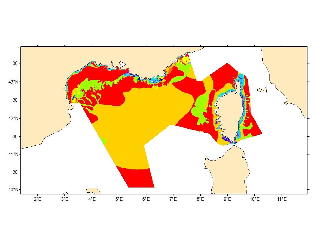
Sediment average grain size in French Mediterranean waters was generated from sediment categories. This rough granulometry estimate may be used for habitat models at meso- and large scale.

'''DEFINITION''' The CMEMS MEDSEA_OMI_tempsal_extreme_var_temp_mean_and_anomaly OMI indicator is based on the computation of the annual 99th percentile of Sea Surface Temperature (SST) from model data. Two different CMEMS products are used to compute the indicator: The Iberia-Biscay-Ireland Multi Year Product (MEDSEA_MULTIYEAR_PHY_006_004) and the Analysis product (MEDSEA_ANALYSISFORECAST_PHY_006_013). Two parameters have been considered for this OMI: * Map of the 99th mean percentile: It is obtained from the Multi Year Product, the annual 99th percentile is computed for each year of the product. The percentiles are temporally averaged over the whole period (1987-2019). * Anomaly of the 99th percentile in 2020: The 99th percentile of the year 2020 is computed from the Near Real Time product. The anomaly is obtained by subtracting the mean percentile from the 2020 percentile. This indicator is aimed at monitoring the extremes of sea surface temperature every year and at checking their variations in space. The use of percentiles instead of annual maxima, makes this extremes study less affected by individual data. This study of extreme variability was first applied to the sea level variable (Pérez Gómez et al 2016) and then extended to other essential variables, such as sea surface temperature and significant wave height (Pérez Gómez et al 2018 and Alvarez Fanjul et al., 2019). More details and a full scientific evaluation can be found in the CMEMS Ocean State report (Alvarez Fanjul et al., 2019). '''CONTEXT''' The Sea Surface Temperature is one of the Essential Ocean Variables, hence the monitoring of this variable is of key importance, since its variations can affect the ocean circulation, marine ecosystems, and ocean-atmosphere exchange processes. As the oceans continuously interact with the atmosphere, trends of sea surface temperature can also have an effect on the global climate. In recent decades (from mid ‘80s) the Mediterranean Sea showed a trend of increasing temperatures (Ducrocq et al., 2016), which has been observed also by means of the CMEMS SST_MED_SST_L4_REP_OBSERVATIONS_010_021 satellite product and reported in the following CMEMS OMI: MEDSEA_OMI_TEMPSAL_sst_area_averaged_anomalies and MEDSEA_OMI_TEMPSAL_sst_trend. The Mediterranean Sea is a semi-enclosed sea characterized by an annual average surface temperature which varies horizontally from ~14°C in the Northwestern part of the basin to ~23°C in the Southeastern areas. Large-scale temperature variations in the upper layers are mainly related to the heat exchange with the atmosphere and surrounding oceanic regions. The Mediterranean Sea annual 99th percentile presents a significant interannual and multidecadal variability with a significant increase starting from the 80’s as shown in Marbà et al. (2015) which is also in good agreement with the multidecadal change of the mean SST reported in Mariotti et al. (2012). Moreover the spatial variability of the SST 99th percentile shows large differences at regional scale (Darmariaki et al., 2019; Pastor et al. 2018). '''CMEMS KEY FINDINGS''' The Mediterranean mean Sea Surface Temperature 99th percentile evaluated in the period 1987-2019 (upper panel) presents highest values (~ 28-30 °C) in the eastern Mediterranean-Levantine basin and along the Tunisian coasts especially in the area of the Gulf of Gabes, while the lowest (~ 23–25 °C) are found in the Gulf of Lyon (a deep water formation area), in the Alboran Sea (affected by incoming Atlantic waters) and the eastern part of the Aegean Sea (an upwelling region). These results are in agreement with previous findings in Darmariaki et al. (2019) and Pastor et al. (2018) and are consistent with the ones presented in CMEMS OSR3 (Alvarez Fanjul et al., 2019) for the period 1993-2016. The 2020 Sea Surface Temperature 99th percentile anomaly map (bottom panel) shows a general positive pattern up to +3°C in the North-West Mediterranean area while colder anomalies are visible in the Gulf of Lion and North Aegean Sea . This Ocean Monitoring Indicator confirms the continuous warming of the SST and in particular it shows that the year 2020 is characterized by an overall increase of the extreme Sea Surface Temperature values in almost the whole domain with respect to the reference period. This finding can be probably affected by the different dataset used to evaluate this anomaly map: the 2020 Sea Surface Temperature 99th percentile derived from the Near Real Time Analysis product compared to the mean (1987-2019) Sea Surface Temperature 99th percentile evaluated from the Reanalysis product which, among the others, is characterized by different atmospheric forcing). Note: The key findings will be updated annually in November, in line with OMI evolutions. '''DOI (product):''' https://doi.org/10.48670/moi-00266

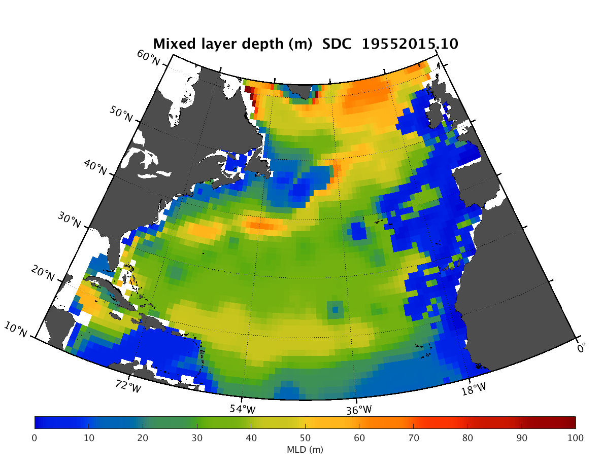
The SDC_NAT_DP1 product contains the North Atlantic Ocean monthly climatology for mixed layer depth (MLD) based on temperature climatology spanning 60 years (1955-2015). The MLD fields have spatial resolution 1/4°. The profiles of temperature combines data from 2 major sources, the SeaDataNet infrastructure and a part of data of the Coriolis Ocean Dataset for Reanalysis (CORA). The used climatology is the SeaDataCloud North Atlantic Ocean Temperature Climatology V1 (https://doi.org/10.13155/61810) done with the DIVA software, version 4.7.2. The product was developed in framework of the SeaDataCloud project. This product must be considered as feasibility study for the next phases, it is a beta-version and that further research needs to be done before its usage from users.

'''DEFINITION''' The global yearly ocean CO2 sink represents the ocean uptake of CO2 from the atmosphere computed over the whole ocean. It is expressed in PgC per year. The ocean monitoring index is presented for the period 1985 to year-1. The yearly estimate of the ocean CO2 sink corresponds to the mean of a 100-member ensemble of CO2 flux estimates (Chau et al. 2022). The range of an estimate with the associated uncertainty is then defined by the empirical 68% interval computed from the ensemble. '''CONTEXT''' Since the onset of the industrial era in 1750, the atmospheric CO2 concentration has increased from about 277±3 ppm (Joos and Spahni, 2008) to 412.44±0.1 ppm in 2020 (Dlugokencky and Tans, 2020). By 2011, the ocean had absorbed approximately 28 ± 5% of all anthropogenic CO2 emissions, thus providing negative feedback to global warming and climate change (Ciais et al., 2013). The ocean CO2 sink is evaluated every year as part of the Global Carbon Budget (Friedlingstein et al. 2022). The uptake of CO2 occurs primarily in response to increasing atmospheric levels. The global flux is characterized by a significant variability on interannual to decadal time scales largely in response to natural climate variability (e.g., ENSO) (Friedlingstein et al. 2022, Chau et al. 2022). '''CMEMS KEY FINDINGS''' The rate of change of the integrated yearly surface downward flux has increased by 0.04±0.01e-1 PgC/yr2 over the period 1985 to year-1. The yearly flux time series shows a plateau in the 90s followed by an increase since 2000 with a growth rate of 0.06±0.04e-1 PgC/yr2. In 2021 (resp. 2020), the global ocean CO2 sink was 2.41±0.13 (resp. 2.50±0.12) PgC/yr. The average over the full period is 1.61±0.10 PgC/yr with an interannual variability (temporal standard deviation) of 0.46 PgC/yr. In order to compare these fluxes to Friedlingstein et al. (2022), the estimate of preindustrial outgassing of riverine carbon of 0.61 PgC/yr, which is in between the estimate by Jacobson et al. (2007) (0.45±0.18 PgC/yr) and the one by Resplandy et al. (2018) (0.78±0.41 PgC/yr) needs to be added. A full discussion regarding this OMI can be found in section 2.10 of the Ocean State Report 4 (Gehlen et al., 2020) and in Chau et al. (2022). '''DOI (product):''' https://doi.org/10.48670/moi-00223

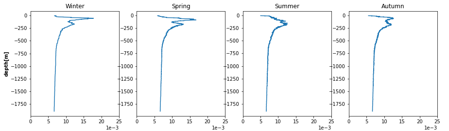
The SDC_GLO_CLIM_N2 product contains seasonally averaged Brunt-Vaisala squared frequency profiles using the density profiles computed in SeadataCloud Global Ocean Climatology - Density Climatology. The Density Climatology product uses the Profiling Floats (PFL) data from World Ocean database 18 for the time period 2003 to 2017 with a Nonlinear Quality procedure applied on it. Computed BVF profiles are averaged seasonally into 5x5 degree boxes for Atlantic and Pacific Oceans. For data access, please register at http://www.marine-id.org/.

Assessments run at AFWG provide the scientific basis for the management of cod, haddock, saithe, redfish, Greenland halibut and capelin in subareas 1 and 2. Taking the catch values provided by the Norwegian fisheries ministry for Norwegian catches1 and raising the total landed value to the total catches gives an approximate nominal first-hand landed value for the combined AFWG stocks of ca. 20 billion NOK or ca. 2 billion EUR (2018 estimates).

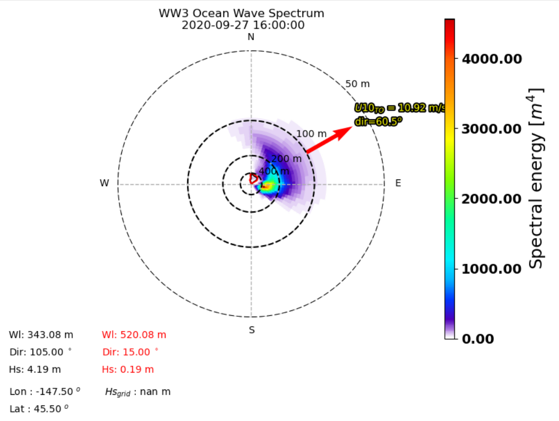
The Ifremer Wind and Wave Operation Center (IWWOC) runs daily the WaveWatch III (WW3) model to provide surface wave colocations with both SCAT and SWIM instruments onboard CFOSAT. CFOSAT (Chinese French Ocean SATellite) is a french-chinese mission launched in 2018, whose aim is to provide wind (SCAT instrument) and wave (SWIM instrument) measurements over the sea surface. Directional wave spectra are calculated over SWIM sensing geometries over each measurement, thanks to the dedicated toolbox (WAVERUN) which was developed by IFREMER for the colocation of WW3 and satellite remote sensing products. The current Ifremer WW3 run is global, hourly and at 0.25° spatial resolution. Two different colocation product are generated: - WW3 with CWWIC L2 provides WW3 directional spectra over the CWWIC SWIM L2 geometry, meaning a colocated valid is provided for each box defined in CWWIC L2 product. - WW3 with IWWOC L2S provides a WW3 directional spectra over IWWOC SWI_L2S__ product. For each of these products, a colocation product is provided respetively for each input file from CWWIC SWI_L2___ and IWWOC SWI_L2S (for each incidence in the later one). It contains the modelled spectral density and all forcing fields: current, wind, friction velocity, air sea temperature difference. Other parameters can be added in the future. The SWIM and WW3 colocation product is generated and distributed by Ifremer / CERSAT in the frame of the Ifremer Wind and Wave Operation Center (IWWOC) co-funded by Ifremer and CNES and dedicated to the processing of the delayed mode data of CFOSAT mission. Note: colocations with SCAT instrument onboard CFOSAT are also within the SWISCA L2S product also available at IWWOC. It provides WW3 directional spectra over SCAT L2A geometry, meaning a model value is calculated for each Wind Vector Cell (WVC) of L2A/L2B types of SCAT product.

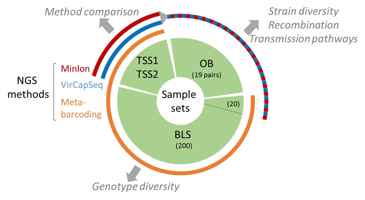
The present data set concerne metabarcoding raw reads produced using 4 different PCR targeting polymerase or capside coding region of the genoyupe I and II of norovirus. Test samples of norovirus with serial dilutions in pure water and after a bio-accumulation in oysters. Sequencing was made after VirCapSeq-VERT approach.

'''DEFINITION''' The Mediterranean water mass formation rates are evaluated in 4 areas as defined in the Ocean State Report issue 2 (OSR2, von Schuckmann et al., 2018) section 3.4 (Simoncelli and Pinardi, 2018): (1) the Gulf of Lions for the Western Mediterranean Deep Waters (WMDW); (2) the Southern Adriatic Sea Pit for the Eastern Mediterranean Deep Waters (EMDW); (3) the Cretan Sea for Cretan Intermediate Waters (CIW) and Cretan Deep Waters (CDW); (4) the Rhodes Gyre, the area of formation of the so-called Levantine Intermediate Waters (LIW) and Levantine Deep Waters (LDW). Annual water mass formation rates have been computed using daily mixed layer depth estimates (density criteria Δσ = 0.01 kg/m3, 10 m reference level) considering the annual maximum volume of water above mixed layer depth with potential density within or higher the specific thresholds specified in Table 1 then divided by seconds per year. Annual mean values are provided using the Mediterranean 1/24o eddy resolving reanalysis (Escudier et al. 2020, 2021). Time spans from 1987 to the year preceding the current one [-1Y], operationally extended yearly. '''CONTEXT''' The formation of intermediate and deep water masses is one of the most important processes occurring in the Mediterranean Sea, being a component of its general overturning circulation. This circulation varies at interannual and multidecadal time scales and it is composed of an upper zonal cell (Zonal Overturning Circulation) and two main meridional cells in the western and eastern Mediterranean (Pinardi and Masetti 2000). The objective is to monitor the main water mass formation events using the eddy resolving Mediterranean Sea Reanalysis (MEDSEA_MULTIYEAR_PHY_006_004, Escudier et al. 2020, 2021) and considering Pinardi et al. (2015) and Simoncelli and Pinardi (2018) as references for the methodology. The Mediterranean Sea Reanalysis can reproduce both Eastern Mediterranean Transient and Western Mediterranean Transition phenomena and catches the principal water mass formation events reported in the literature. This will permit constant monitoring of the open ocean deep convection process in the Mediterranean Sea and a better understanding of the multiple drivers of the general overturning circulation at interannual and multidecadal time scales. Deep and intermediate water formation events reveal themselves by a deep mixed layer depth distribution in four Mediterranean areas: Gulf of Lions, Southern Adriatic Sea Pit, Cretan Sea and Rhodes Gyre. '''KEY FINDINGS''' The Western Mediterranean Deep Water (WMDW) formation events in the Gulf of Lion appear to be larger after 1999 consistently with Schroeder et al. (2006, 2008) related to the Eastern Mediterranean Transient event. This modification of WMDW after 2005 has been called Western Mediterranean Transition. WMDW formation events are consistent with Somot et al. (2016) and the event in 2009 is also reported in Houpert et al. (2016). The Eastern Mediterranean Deep Water (EMDW) formation in the Southern Adriatic Pit region displays a period of water mass formation between 1988 and 1993, in agreement with Pinardi et al. (2015), in 1996, 1999 and 2000 as documented by Manca et al. (2002). Weak deep water formation in winter 2006 is confirmed by observations in Vilibić and Šantić (2008). An intense deep water formation event is detected in 2012-2013 (Gačić et al., 2014). Last years are characterized by large events starting from 2017 (Mihanovic et al., 2021). Cretan Intermediate Water formation rates present larger peaks between 1989 and 1993 with the ones in 1992 and 1993 composing the Eastern Mediterranean Transient phenomena. The Cretan Deep Water formed in 1992 and 1993 is characterized by the highest densities of the entire period in accordance with Velaoras et al. (2014). The Levantine Deep Water formation rate in the Rhode Gyre region presents the largest values between 1992 and 1993 in agreement with Kontoyiannis et al. (1999). '''DOI (product):''' https://doi.org/10.48670/mds-00318