Moving 6-year analysis of Water body silicate in the Mediterranean Sea for each season: - winter: January-March, - spring: April-June, - summer: July-September, - autumn: October-December. Every year of the time dimension corresponds to the 6-year centered average of the season. 6-years periods span from 1970-1975 until 2018-2023. Description of DIVA analysis: The computation was done with the DIVAnd (Data-Interpolating Variational Analysis in n dimensions), version 2.7.12, using GEBCO 30sec topography for the spatial connectivity of water masses. The horizontal resolution of the produced DIVAnd maps grids is dx=dy=0.125 degrees (around 13.5km and 10.9km accordingly). The vertical resolution is 25 depth levels: [0.,5.,10.,20.,30.,50.,75.,100.,125.,150.,200.,250.,300.,400.,500.,600.,700.,800.,900.,1000.,1100.,1200.,1300.,1400.,1500.]. The horizontal correlation length is 200km. The vertical correlation length (in meters) was set twices the vertical resolution: [10.,10.,20.,20.,40.,50.,50.,50.,50.,100.,100.,100.,200.,200.,200.,200.,200.,200.,200.,200.,200.,200.,200.,200.,200.]. Duplicates check was performed using the following criteria for space and time: dlon=0.001deg., dlat=0.001deg., ddepth=1m, dtime=1hour, dvalue=0.1. The error variance (epsilon2) was set equal to 1 for profiles and 10 for time series to reduce the influence of close data near the coasts. An anamorphosis transformation was applied to the data (function DIVAnd.Anam.loglin) to avoid unrealistic negative values: threshold value=200. A background analysis field was used for all years (1970-2023) with correlation length equal to 600km and error variance (epsilon2) equal to 20. Quality control of the observations was applied using the interpolated field (QCMETHOD=3). Residuals (differences between the observations and the analysis (interpolated linearly to the location of the observations) were calculated. Observations with residuals outside the minimum and maximum values of the 99% quantile were discarded from the analysis. Originators of Italian data sets-List of contributors: - Brunetti Fabio (OGS) - Cardin Vanessa, Bensi Manuel doi:10.6092/36728450-4296-4e6a-967d-d5b6da55f306 - Cardin Vanessa, Bensi Manuel, Ursella Laura, Siena Giuseppe doi:10.6092/f8e6d18e-f877-4aa5-a983-a03b06ccb987 - Cataletto Bruno (OGS) - Cinzia Comici Cinzia (OGS) - Civitarese Giuseppe (OGS) - DeVittor Cinzia (OGS) - Giani Michele (OGS) - Kovacevic Vedrana (OGS) - Mosetti Renzo (OGS) - Solidoro C.,Beran A.,Cataletto B.,Celussi M.,Cibic T.,Comici C.,Del Negro P.,De Vittor C.,Minocci M.,Monti M.,Fabbro C.,Falconi C.,Franzo A.,Libralato S.,Lipizer M.,Negussanti J.S.,Russel H.,Valli G., doi:10.6092/e5518899-b914-43b0-8139-023718aa63f5 - Celio Massimo (ARPA FVG) - Malaguti Antonella (ENEA) - Fonda Umani Serena (UNITS) - Bignami Francesco (ISAC/CNR) - Boldrini Alfredo (ISMAR/CNR) - Marini Mauro (ISMAR/CNR) - Miserocchi Stefano (ISMAR/CNR) - Zaccone Renata (IAMC/CNR) - Lavezza, R., Dubroca, L. F. C., Ludicone, D., Kress, N., Herut, B., Civitarese, G., Cruzado, A., Lefèvre, D.,Souvermezoglou, E., Yilmaz, A., Tugrul, S., and Ribera d'Alcala, M.: Compilation of quality controlled nutrient profiles from the Mediterranean Sea, doi:10.1594/PANGAEA.771907, 2011.

This dataset contains the dynamical outputs of a global ocean simulation coupling dynamics and biogeochemistry at ¼° over the year 2019. The simulation has been performed using the coupled circulation/ecosystem model NEMO/PISCES (https://www.nemo-ocean.eu/), which is here enhanced to perform an ensemble simulation with explicit simulation of modeling uncertainties in the physics and in the biogeochemistry. This dataset is one of the 40 members of the ensemble simulation. This study was part of the Horizon Europe project SEAMLESS (https://seamlessproject.org/Home.html), with the general objective of improving the analysis and forecast of ecosystem indicators.   See Popov et al. (https://os.copernicus.org/articles/20/155/2024/) for more details on the study.

The Southern Ocean plays a fundamental role in regulating the global climate. This ocean also contains a rich and highly productive ecosystem, potentially vulnerable to climate change. Very large national and international efforts are directed towards the modeling of physical oceanographic processes to predict the response of the Southern Ocean to global climate change and the role played by the large-scale ocean climate processes. However, these modeling efforts are greatly limited by the lack of in situ measurements, especially at high latitudes and during winter months. The standard data that are needed to study ocean circulation are vertical profiles of temperature and salinity, from which we can deduce the density of seawater. These are collected with CTD (Conductivity-Temperature-Depth) sensors that are usually deployed on research vessels or, more recently, on autonomous Argo profilers. The use of conventional research vessels to collect these data is very expensive, and does not guarantee access to areas where sea ice is found at the surface of the ocean during the winter months. A recent alternative is the use of autonomous Argo floats. However, this technology is not easy to use in glaciated areas. In this context, the collection of hydrographic profiles from CTDs mounted on marine mammals is very advantageous. The choice of species, gender or age can be done to selectively obtain data in particularly under-sampled areas such as under the sea ice or on continental shelves. Among marine mammals, elephant seals are particularly interesting. Indeed, they have the particularity to continuously dive to great depths (590 ± 200 m, with maxima around 2000 m) for long durations (average length of a dive 25 ± 15 min, maximum 80 min). A Conductivity-Temperature-Depth Satellite Relay Data Logger (CTD-SRDLs) has been developed in the early 2000s to sample temperature and salinity vertical profiles during marine mammal dives (Boehme et al. 2009, Fedak 2013). The CTD-SRDL is attached to the seal on land, then it records hydrographic profiles during its foraging trips, sending the data by satellite ARGOS whenever the seal goes back to the surface.While the principle intent of seal instrumentation was to improve understanding of seal foraging strategies (Biuw et al., 2007), it has also provided as a by-product a viable and cost-effective method of sampling hydrographic properties in many regions of the Southern Ocean (Charrassin et al., 2008; Roquet et al., 2013).

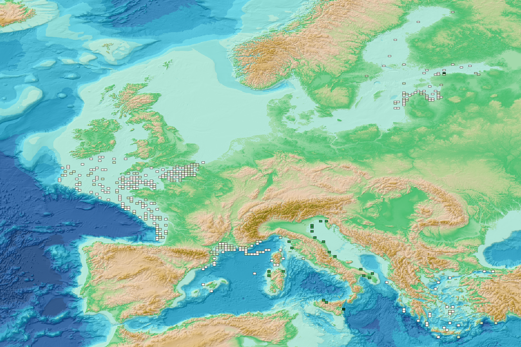
The ICES Working Group on Fisheries Benthic Impact and Trade-offs (WGFBIT) has developed an assessment framework based on the life history trait longevity, to evaluate the benthic impact of fisheries at the regional scale. In order to apply this framework to the Mediterranean sea, several Mediterranean longevity databases were merged together with existing North-East Atlantic ones to develop a common database. Longevity was fuzzy coded into four longevity classes: <1, 1-3, 3-10 and >10 years. Both benthic mega and macrofauna organisms are included in this dataset. Further details about both the purpose and the methodology may be found in ICES (2022) and Cuyvers et al. (2023). The result of the final dataset merging is one dataset containing the fuzzy coded average longevity (and standard deviation) for 2264 taxa and for each, the number of databases used. 

This visualization product displays beaches locations where the Marine Strategy Framework Directive (MSFD) monitoring protocol has been applied to collate data on macrolitter (> 2.5 cm). Reference lists associated with these protocols have been indicated with different colors in the map. EMODnet Chemistry included the collection of marine litter in its 3rd phase. Since the beginning of 2018, data of beach litter have been gathered and processed in the EMODnet Chemistry Marine Litter Database (MLDB). The harmonization of all the data has been the most challenging task considering the heterogeneity of the data sources, sampling protocols and reference lists used on a European scale. Preliminary processings were necessary to harmonize all the data: - Exclusion of OSPAR 1000 protocol: in order to follow the approach of OSPAR that it is not including these data anymore in the monitoring; - Selection of MSFD surveys only (exclusion of other monitoring, cleaning and research operations); - Exclusion of beaches without coordinates; - Some categories & some litter types like organic litter, small fragments (paraffin and wax; items > 2.5cm) and pollutants have been removed. This list was created using EU Marine Beach Litter Baselines, the European Threshold Value for Macro Litter on Coastlines and the Joint list of litter categories for marine macro-litter monitoring from JRC (these three documents are attached to this metadata). More information is available in the attached documents. Warning: the absence of data on the map does not necessarily mean that they do not exist, but that no information has been entered in the Marine Litter Database for this area.

This set of data documents the radiocarbon dates (n=19) obtained thanks to the accelerator mass spectrometry method (AMS) at the LMC14/ARTEMIS French national facility on the cores (Multicorer, Kullenberg) retrieved from the West-Gironde mud patch (WGMP) during the JERICObent-7 cruise (10-15 July 2019; NR Côtes de la Manche, https://doi.org/10.17600/18001022). The WGMP registers very high sedimentation rates since the last 600 years (≥ 0.3 cm/yr) and is thus of great interest for palaeoceanographic investigations. At present, this depocenter marks the mid-shelf of the temperate Bay of Biscay off major French rivers from the Aquitaine basin. The fine mud deposits of the WGMP are of 3 to 4 meters thick and lie on palimpsest levels rich in gravels and shells. They cover a V-shaped structure, oriented SW-NE, which is attributed to the incision(s) of a paleovalley in the Cenozoic substrate, mainly linked to the paleo-Gironde routing changes during past glacials/interglacials, and its potential past convergences with the paleo-rivers of the Antioche perthuis (Seudre, Charente paleovalleys?) at that times. Detailed information on each sample is presented with the 14C results obtained by the Artemis AMS facility at LMC14 laboratory (Dumoulin et al. 2017- https://doi.org/10.1017/RDC.2016.116, Beck et al. 2024- https://doi.org/10.1017/RDC.2023.23). Raw ages are indicated together with calibration calculations using the last two versions of the Calib software (http://calib.org/, Calib 7 and 8) to show the dispersion of ages linked to the updating of calibration curves (Marine13, Intcal13, Marine20, Intcal 20). The calibrated ages finally retained for publications (used in the related Seanoe document - https://doi.org/10.17882/104237 - and published in Eynaud et al., 2025 for the ST3c core, https://doi.org/10.1016/j.gloplacha.2025.105039) are those obtained with the last Calib 8.1 version. Raw 14C ages were calibrated and converted to calendar ages using the IntCal20 calibration curve with a reservoir age correction of 400 years deduced from Radionuclide analyses (137Cs and 210Pb) at the top of the studied cores (see Schmidt, 2025, https://www.seanoe.org/data/00968/107979/). 

Sardine physiological measurments from september to november 2020

EMODnet Chemistry aims to provide access to marine chemistry datasets and derived data products concerning eutrophication, acidity and contaminants. The importance of the selected substances and other parameters relates to the Marine Strategy Framework Directive (MSFD). This aggregated dataset contains all unrestricted EMODnet Chemistry data on eutrophication and acidity, and covers the Mediterranean Sea. Data were aggregated and quality controlled by the 'Hellenic Centre for Marine Research, Hellenic National Oceanographic Data Centre (HCMR/HNODC)' in Greece. ITS-90 water temperature and water body salinity variables have also been included ('as are') to complete the eutrophication and acidity data. If you use these variables for calculations, please refer to SeaDataNet for the quality flags: https://www.seadatanet.org/Products/Aggregated-datasets. Regional datasets concerning eutrophication and acidity are automatically harvested, and the resulting collections are aggregated and quality controlled using ODV Software and following a common methodology for all sea regions (https://doi.org/10.13120/8xm0-5m67 ) Parameter names are based on P35 vocabulary, which relates to EMODnet Chemistry aggregated parameter names and is available at: https://vocab.nerc.ac.uk/search_nvs/P35/. When not present in original data, water body nitrate plus nitrite was calculated by summing all nitrate and nitrite parameters. The same procedure was applied for water body dissolved inorganic nitrogen (DIN), which was calculated by summing all nitrate, nitrite, and ammonium parameters. Concentrations per unit mass were converted to a unit volume using a constant density of 1.025 kg/L. The aggregated dataset can also be downloaded as an ODV collection and spreadsheet, which is composed of a metadata header followed by tab separated values. This spreadsheet can be imported to ODV Software for visualisation (more information can be found at: https://www.seadatanet.org/Software/ODV ).

'''DEFINITION''' The temporal evolution of thermosteric sea level in an ocean layer is obtained from an integration of temperature driven ocean density variations, which are subtracted from a reference climatology to obtain the fluctuations from an average field. The products used include three global reanalyses: GLORYS, C-GLORS, ORAS5 (GLOBAL_MULTIYEAR_PHY_ENS_001_031) and two in situ based reprocessed products: CORA5.2 (INSITU_GLO_PHY_TS_OA_MY_013_052) , ARMOR-3D (MULTIOBS_GLO_PHY_TSUV_3D_MYNRT_015_012). The regional thermosteric sea level values are then averaged from 60°S-60°N aiming to monitor interannual to long term global sea level variations caused by temperature driven ocean volume changes through thermal expansion as expressed in meters (m). '''CONTEXT''' Most of the interannual variability and trends in regional sea level is caused by changes in steric sea level. At mid and low latitudes, the steric sea level signal is essentially due to temperature changes, i.e. the thermosteric effect (Stammer et al., 2013, Meyssignac et al., 2016). Salinity changes play only a local role. Regional trends of thermosteric sea level can be significantly larger compared to their globally averaged versions (Storto et al., 2018). Except for shallow shelf sea and high latitudes (> 60° latitude), regional thermosteric sea level variations are mostly related to ocean circulation changes, in particular in the tropics where the sea level variations and trends are the most intense over the last two decades. '''CMEMS KEY FINDINGS''' Significant (i.e. when the signal exceeds the noise) regional trends for the period 2005-2023 from the Copernicus Marine Service multi-ensemble approach show a thermosteric sea level rise at rates ranging from the global mean average up to more than 8 mm/year. There are specific regions where a negative trend is observed above noise at rates up to about -5 mm/year such as in the subpolar North Atlantic, or the western tropical Pacific. These areas are characterized by strong year-to-year variability (Dubois et al., 2018; Capotondi et al., 2020). Note: The key findings will be updated annually in November, in line with OMI evolutions. '''DOI (product):''' https://doi.org/10.48670/moi-00241

The ESA Sea State Climate Change Initiative (CCI) project has produced global multi-sensor time-series of along-track satellite altimeter significant wave height data (referred to as Level 2P (L2P) data) with a particular focus for use in climate studies. This dataset contains the Version 4 Remote Sensing Significant Wave Height product, which provides along-track data at approximately 6 km spatial resolution, separated per satellite and pass, including all measurements with flags, bias corrections and extra parameters from other sources. These are expert products with rich content and no data loss. The altimeter data used in the Sea State CCI dataset v4 come from multiple satellite missions spanning from 1992 to 2023 (ERS-1, ERS-2, Envisat, CryoSat-2, Jason-1, Jason-2, Jason-3, SARAL, Sentinel-3 A, Sentinel-3 B, Sentinel-6 A), therefore spanning over a larger time range than the previous version 3. The missions already retracked (with WHALES) in version 3 were not reprocessed, but extended when applicable. Many altimeters are bi-frequency (Ku-C or Ku-S) and only measurements in Ku band were used, for consistency reasons, being available on each altimeter but SARAL (Ka band). **The version 4 of this dataset now supersedes the previous version 3.**