 Catalogue PIGMA
2023
Type of resources
Available actions
Topics
Keywords
Contact for the resource
Provided by
Years
Formats
Representation types
Update frequencies
status
Scale
Resolution
-
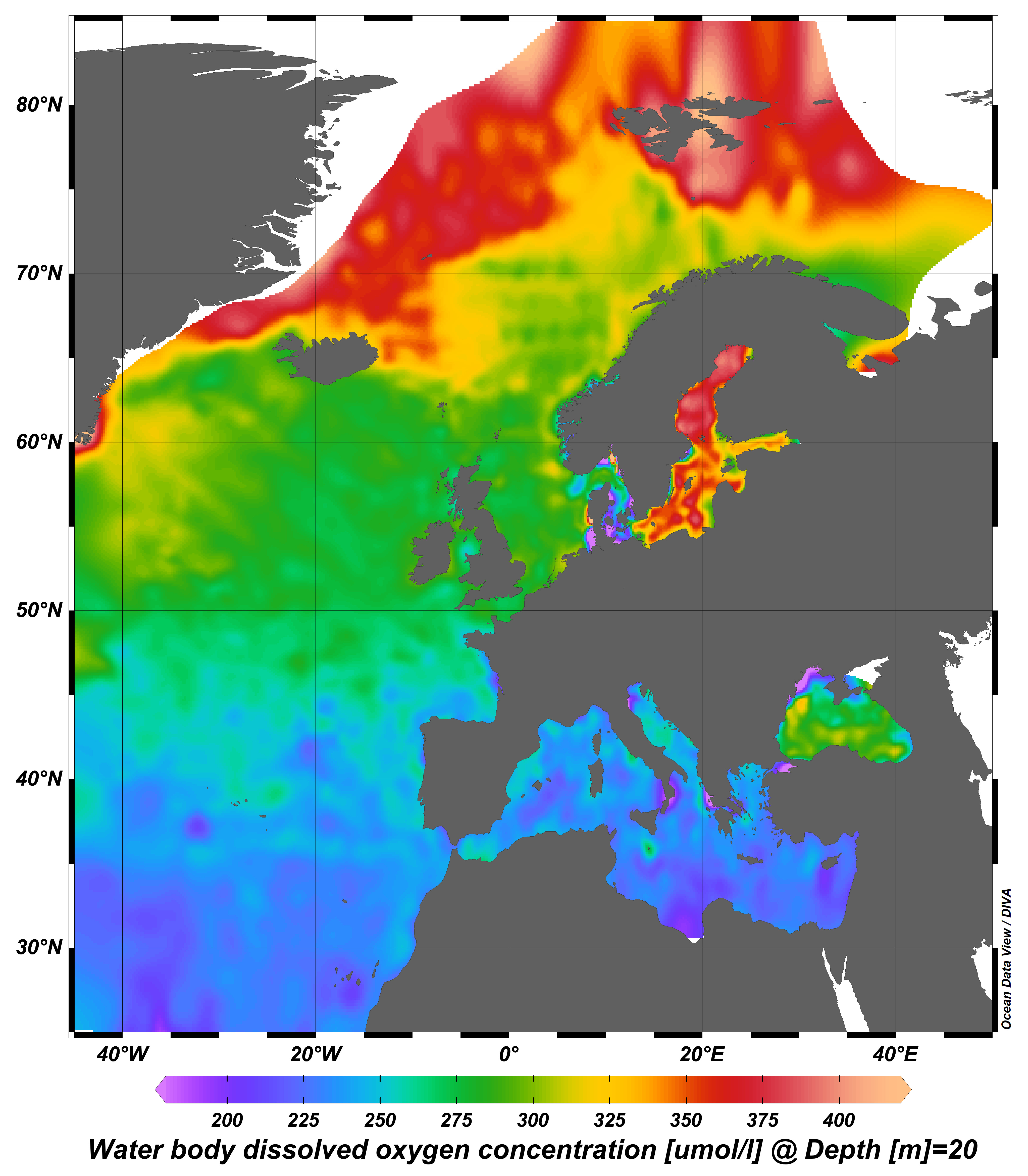
Water body ammonium - Monthly Climatology for the European Seas for the period 1960-2020 on the domain from longitude -45.0 to 70.0 degrees East and latitude 24.0 to 83.0 degrees North. Data Sources: observational data from SeaDataNet/EMODnet Chemistry Data Network. Description of DIVA analysis: The computation was done with the DIVAnd (Data-Interpolating Variational Analysis in n dimensions), version 2.7.9, using GEBCO 30sec topography for the spatial connectivity of water masses. Horizontal correlation length and vertical correlation length vary spatially depending on the topography and domain. Depth range: 0.0, 5.0, 10.0, 15.0, 20.0, 25.0, 30.0, 35.0, 40.0, 45.0, 50.0, 55.0, 60.0, 65.0, 70.0, 75.0, 80.0, 85.0, 90.0, 95.0, 100.0, 125.0, 150.0, 175.0, 200.0, 225.0, 250.0, 275.0, 300.0, 325.0, 350.0, 375.0, 400.0, 425.0, 450.0, 475.0, 500.0, 550.0, 600.0, 650.0, 700.0, 750.0, 800.0, 850.0, 900.0, 950.0, 1000.0, 1050.0, 1100.0, 1150.0, 1200.0, 1250.0, 1300.0, 1350.0, 1400.0, 1450.0, 1500.0, 1550.0, 1600.0, 1650.0, 1700.0, 1750.0, 1800.0, 1850.0, 1900.0, 1950.0, 2000.0, 2100.0, 2200.0, 2300.0, 2400.0, 2500.0, 2600.0, 2700.0, 2800.0, 2900.0, 3000.0, 3100.0, 3200.0, 3300.0, 3400.0, 3500.0, 3600.0, 3700.0, 3800.0, 3900.0, 4000.0, 4100.0, 4200.0, 4300.0, 4400.0, 4500.0, 4600.0, 4700.0, 4800.0, 4900.0, 5000.0, 5100.0, 5200.0, 5300.0, 5400.0, 5500.0 m. Units: umol/l. The horizontal resolution of the produced DIVAnd analysis is 0.25 degrees.
-
webODV visualisations via WMS from the harmonized, standardized, validated data collections that EMODnet Chemistry is regularly producing and publishing for all European sea basins for eutrophication and contaminants. You can analyze, visualize, subset and download EMODnet Chemistry data using interactive webODV services. More information at: https://emodnet.ec.europa.eu/en/chemistry#chemistry-services
-
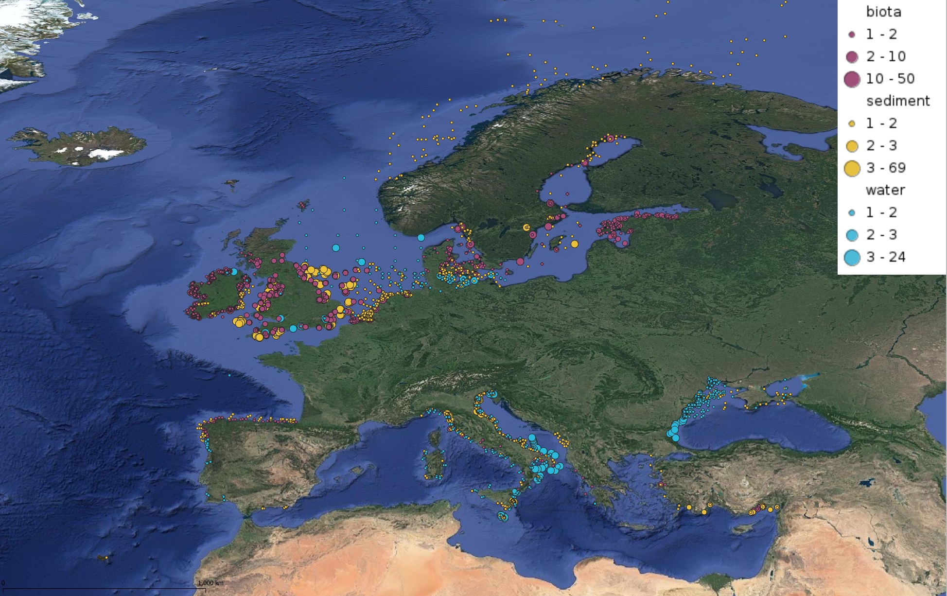
This product displays for Hexachlorobenzene, positions with values counts that have been measured per matrix for each year and are present in EMODnet regional contaminants aggregated datasets, v2022. The product displays positions for every available year.
-
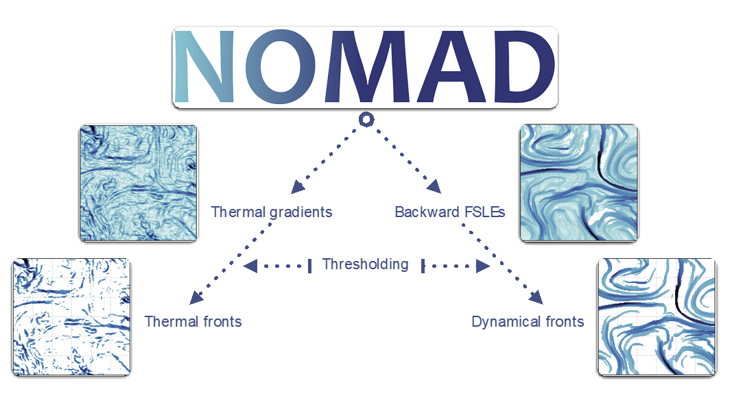
Fronts are ubiquitous discrete features of the global ocean often associated with enhanced vertical velocities, in turn boosting primary production and so forth. Fronts thus form dynamical and ephemeral ecosystems where numerous species meet across all trophic levels. Fronts are also targeted by fisheries. Capturing ocean fronts and studying their long-term variability in relation with climate change is thus key for marine resource management and spatial planning. The Mediterranean Sea and the Southwest Indian Ocean are natural laboratories to study front-marine life interactions due to their energetic flow at sub-to-mesoscales, high biodiversity (including endemic and endangered species) and numerous conservation initiatives. Based on remotely-sensed Sea Surface Temperature and Height, we compute thermal fronts (2003-2020) and attracting Lagrangian Coherent Structures (1994-2020), in both regions over several decades. We advocate for the combined use of both thermal fronts and attracting Lagrangian Coherent Structures to study front-marine life interactions. The resulting front database differs from other alternatives by its high spatio-temporal resolution, long time coverage, and relevant thresholds defined for ecological provinces.
-
Seawater samples (500 mL) were taken during the PIRATA FR-32 cruise to measure surface inorganic carbon and alkalinity. The analyses were realised by potentiometric titration using a closed-cell at the SNAPO-CO2, LOCEAN in Paris.
-

Species distribution models (Random Forest) predicting the distribution of mixed cold-water coral community (Coral Garden) assemblage in the Celtic Sea. This community is considered ecologically coherent according to the cluster analysis conducted by Parry et al. (2015) on image sample. Modelling its distribution complements existing work on their definition and offers a representation of the extent of the areas of the North East Atlantic where they can occur based on the best available knowledge. This work was performed at the University of Plymouth in 2021.
-

This dataset contains libraries of 3 coral species: Acropora hyacinthus, Porites lobata and Poscillopora acuta. In three islands with contrasting thermal regimes, the three species were sampled and brought back to the laboratory to induce an experimental thermal stress. The different colonies were split into two conditions. One part was placed in tanks filled with seawater at a given control temperature, the other part in tanks where the water temperature was increased. The samples in this dataset correspond to part of the control condition samples from French Polynesia and New Caledonia.
-
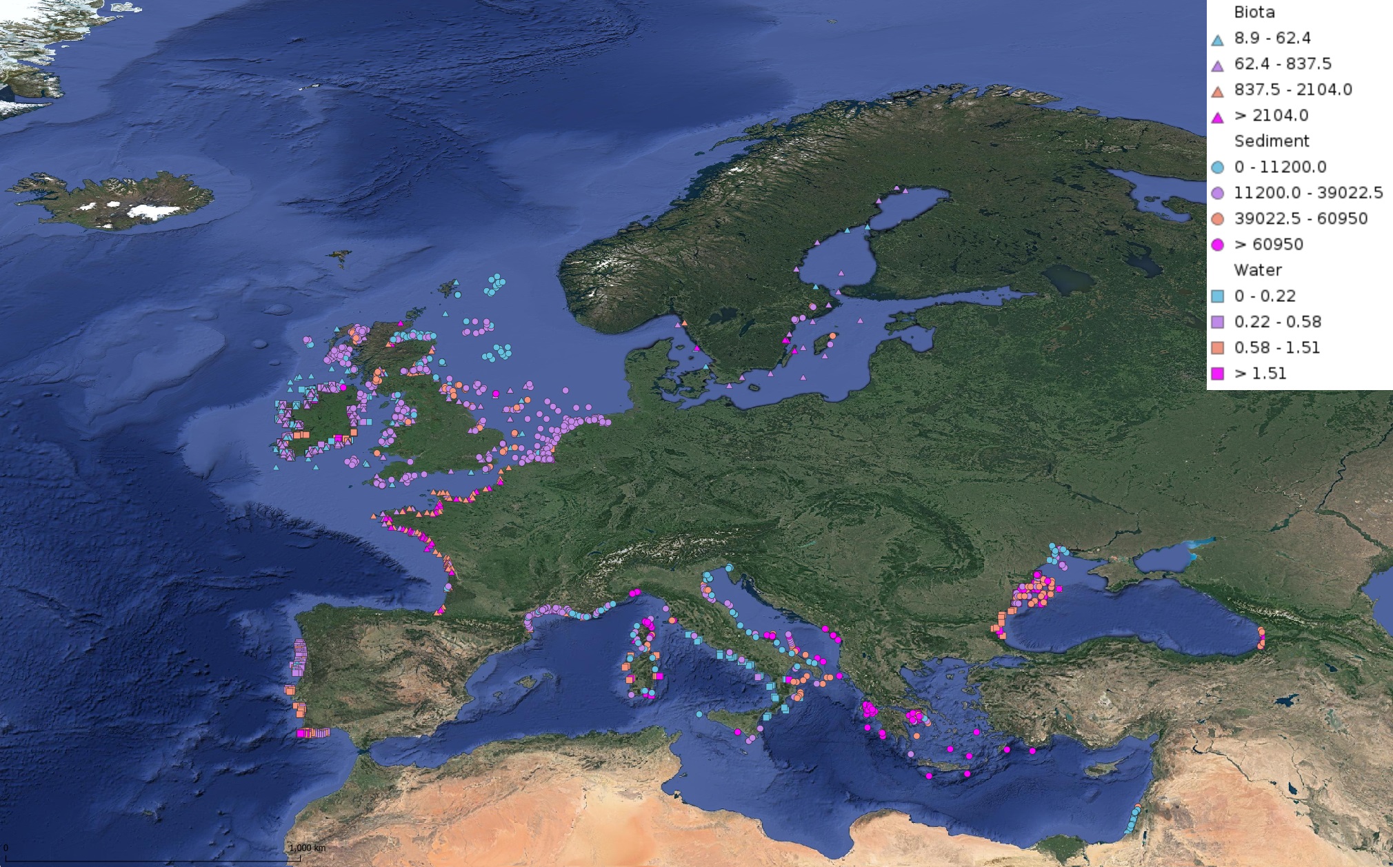
This product displays for Nickel, median values of the last 6 available years that have been measured per matrix and are present in EMODnet regional contaminants aggregated datasets, v2022. The median values ranges are derived from the following percentiles: 0-25%, 25-75%, 75-90%, >90%. Only "good data" are used, namely data with Quality Flag=1, 2, 6, Q (SeaDataNet Quality Flag schema). For water, only surface values are used (0-15 m), for sediment and biota data at all depths are used.
-

Opportunistic macroalgae blooms (green tides) data are collected during monitoring surveys on the English Channel / Bay of Biscay French coasts since 2008 (Quadrige program code : BLOOMS). Protocols are implemented in the European Water Framework Directive.
-
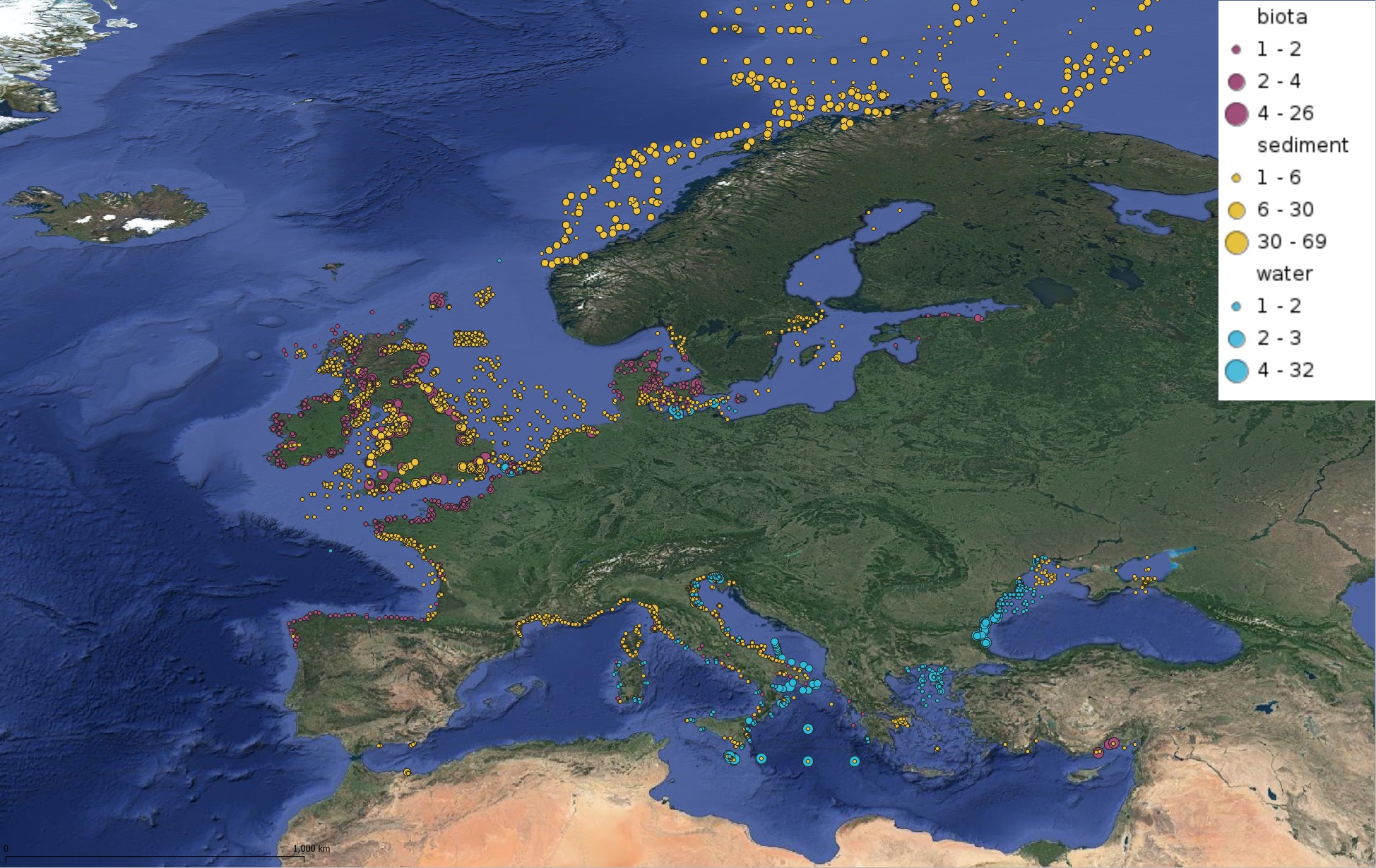
This product displays for Fluoranthene, positions with values counts that have been measured per matrix for each year and are present in EMODnet regional contaminants aggregated datasets, v2022. The product displays positions for every available year.