Web Map Service for Emodnet Chemistry

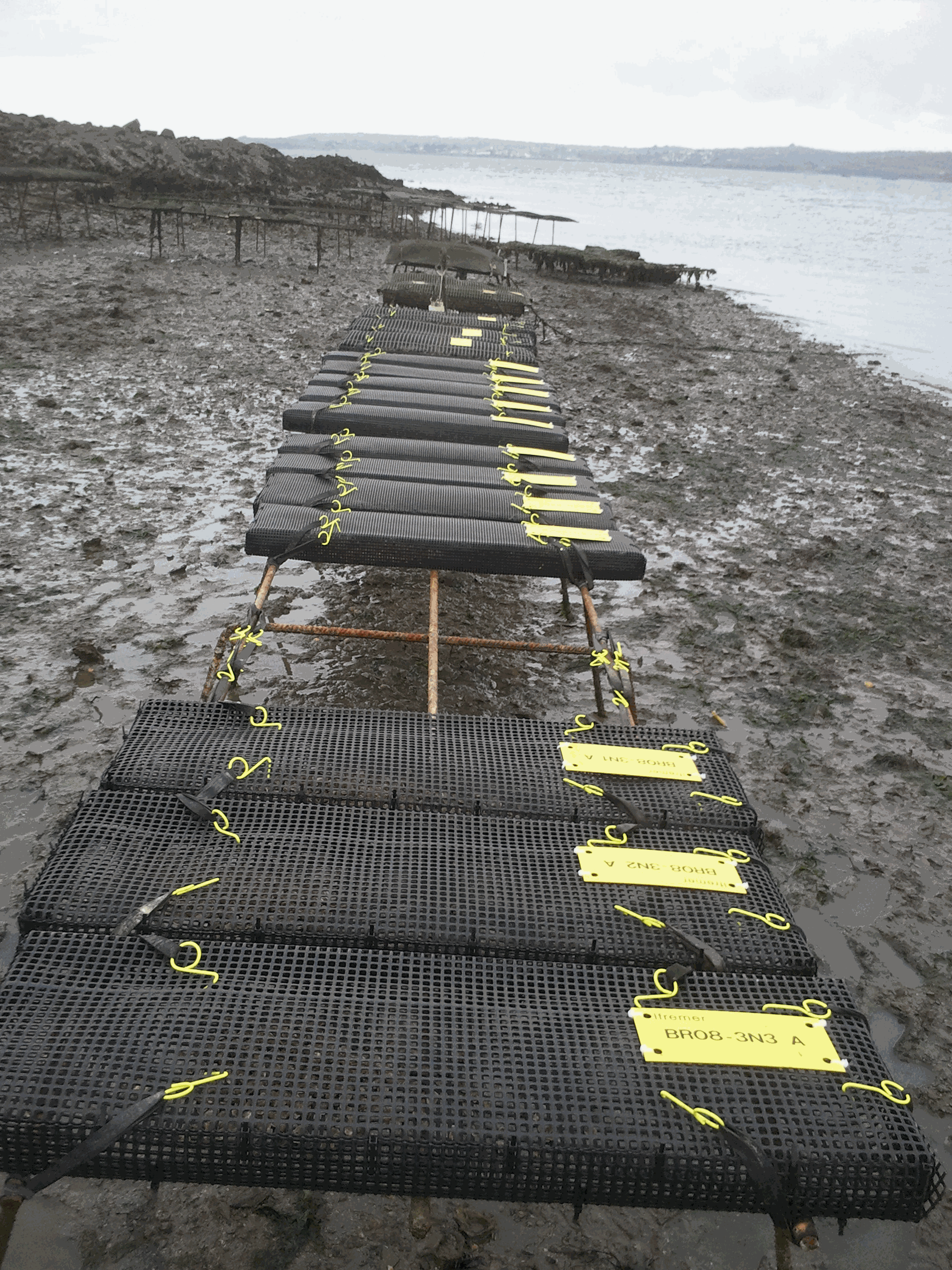
The network was initiated by IFREMER from 1993 to 2009 (under the acronym REMORA) to study the rearing performance of the Pacific oyster Crassostrea gigas at a national scale. To do so, the network monitored annually the mortality and growth of standardized batches of 18-month-old oysters. Starting in 1995, the monitoring of the rearing performance of 6-month-old oyster spat was integrated into this network. These sentinel batches were distributed simultaneously each year on 43 sites and were monitored quarterly. These sites were distributed over the main French oyster farming areas and allowed a national coverage of the multiannual evolution of oyster farming performances. Most of the sites were located on the foreshore at comparable levels of immersion. Field studies were carried out by the "Laboratoires Environnement Ressources" (LER) for the sites included in their geographical area of investigation. Following the increase in spat mortality in 2008, the network evolved in 2009 (under the acronym RESCO). From this date, the network selected 13 sites among the 43 sites previously monitored in order to increase the frequency of visits (twice a month) and the number of sentinel batches. More precisely, sentinel batches of oysters corresponding to different origins (wild or hatchery, diploid or triploid) and to two rearing age classes (spat or 18-month-old adults) were selected. The monitoring of environmental variables (temperature, salinity) associated with the 13 sites was also implemented. The actions of the network have thus contributed to disentangle the biotic and abiotic parameters involved in mortality phenomena, taking into account the different compartments (environment / host / infectious agents) likely to interact with the evolution of oyster rearing performance. Finally, since 2015, the network has merged the RESCO and VELYGER networks to adopt the acronym ECOSCOPA. The general objective of this current network is to analyze the causes of spatio-temporal variability of the main life traits (Larval stage - Recruitment - Reproduction - Growth - Survival - Cytogenetic abnormalities) of the cupped oyster in France and to follow their evolution on the long term in the context of climate change. To do this, the network proposes a regular spatio-temporal monitoring of the major proxies of the life cycle of the oyster, organized in three major thematic groups: (1) proxies related to growth, physiological tolerance and survival of experimental sentinel populations over 3 age classes: (2) proxies related to reproduction, larval phase and recruitment of the species throughout its natural range in France, and: (3) proxies related to environmental parameters essential to the species (weather conditions, temperature, salinity, pH, turbidity, chlorophyll a and phytoplankton) at daily or sub-hourly frequencies. Working in a geographical network associating several laboratories, ECOSCOPA provide these monitoring within 8 sites selected among the previous ones to ensure the continuity of the data acquisition. Today, these 8 sites are considered as ecosystems of common interest, contrasted, namely : - The Thau lagoon - The Arcachon basin - The Marennes Oléron basin - The Bourgneuf Bay - The bay of Vilaine - The bay of Brest - The bay of Mont Saint Michel - The bay of Veys The ECOSCOPA network is therefore one of the relevant monitoring tools on a national scale, allowing to objectively measure through different proxies the general state of health of cultivated and wild oyster populations, and this for the different sensitive phases of their life cycle. This network aims at allowing a better evaluation, on the long term, of the biological risks incurred by the sector but also by the ecosystems, in particular under the increasing constraint of climatic and anthropic changes. Figure : Sites monitored by the ECOSCOPA network  

This dataset contains mesoscale eddies from the Ocean Eddy Detection and Tracking Algorithms (TOEddies) Atlas colocated with Argo profiling floats. Applied to daily gridded maps of satellite Absolute Dynamic Topography, TOEddies provides information on eddy dynamical characteristics (e.g., size and intensity) over a 30+ year period (1993–2023) and identifies complex eddy-eddy interactions that lead to eddy splitting and merging. Furthermore, these eddies are combined with 23 years of Argo profile co-located measurements (2000–2023), enabling investigation into the signature of eddies and their impact in the ocean interior. This dataset contains eddies detected across the entire geographical area covered by altimetric maps. Special caution is advised for studies focusing on eddies near the equator, where geostrophic balance breaks down, and at high latitudes, where the small Rossby radius limits detection capabilities in 1/4° altimetric fields. TOEddies, based on the method proposed and developed by Chaigneau et al. (2008, 2011) and Pegliasco et al. (2018), was first presented in Laxenaire et al. (2018) when applied to the South Atlantic Ocean. To date, approximately 20 peer-reviewed publications have employed the TOEddies algorithm (see Ioannou et al., Preprint 2024 for a recent list of some of them). Notably, mesoscale eddies from TOEddies, following Chaigneau et al. (2011), have been colocated with Argo floats, facilitating, for example, the identification of the transition from surface to subsurface intensified eddies (Laxenaire et al., 2019), the estimation of heat transport by eddies (Laxenaire et al., 2020), and the study of the impact of mesoscale eddies on Deep Chlorophyll Maxima with BGC Argo floats (Cornec et al., 2021). The V1 version of this dataset is described in detail in the appendix of Ioannou et al. (Preprint 2024) and compared to other eddy detection datasets in the core text of Ioannou et al. (Preprint 2024). Input Fields => Satellite Altimetry: Daily all-satellite sea surface height fields produced by Copernicus Marine Service (https://marine.copernicus.eu/fr). This multi-satellite product integrates data from all available satellites at a given time and is projected onto a fixed grid with a resolution of 0.25°, covering the global ocean (version: cmems_obs-sl_glo_phy-ssh_my_allsat-l4-duacs-0.25deg_P1D, DOI:10.48670/moi-00148). Argo Floats: Argo float profile data and positions were retrieved from the Ifremer FTP (Argo, 2024; DOI:10.17882/42182). See Detection eddies repository for technical guidance on this dataset.

EMODnet Chemistry aims to provide access to marine chemistry datasets and derived data products concerning eutrophication, acidity and contaminants. The importance of the selected substances and other parameters relates to the Marine Strategy Framework Directive (MSFD). This aggregated dataset contains all unrestricted EMODnet Chemistry data on eutrophication and acidity, and covers the Mediterranean Sea. Data were aggregated and quality controlled by the 'Hellenic Centre for Marine Research, Hellenic National Oceanographic Data Centre (HCMR/HNODC)' in Greece. ITS-90 water temperature and water body salinity variables have also been included ('as are') to complete the eutrophication and acidity data. If you use these variables for calculations, please refer to SeaDataNet for the quality flags: https://www.seadatanet.org/Products/Aggregated-datasets. Regional datasets concerning eutrophication and acidity are automatically harvested, and the resulting collections are aggregated and quality controlled using ODV Software and following a common methodology for all sea regions (https://doi.org/10.13120/8xm0-5m67 ) Parameter names are based on P35 vocabulary, which relates to EMODnet Chemistry aggregated parameter names and is available at: https://vocab.nerc.ac.uk/search_nvs/P35/. When not present in original data, water body nitrate plus nitrite was calculated by summing all nitrate and nitrite parameters. The same procedure was applied for water body dissolved inorganic nitrogen (DIN), which was calculated by summing all nitrate, nitrite, and ammonium parameters. Concentrations per unit mass were converted to a unit volume using a constant density of 1.025 kg/L. The aggregated dataset can also be downloaded as an ODV collection and spreadsheet, which is composed of a metadata header followed by tab separated values. This spreadsheet can be imported to ODV Software for visualisation (more information can be found at: https://www.seadatanet.org/Software/ODV ).

This dataset contains (1) outputs of Species Distribution Models (SDMs) for marine fish and (2) estimation of species richness using those outputs. SDMs use correlative algorithms to link presences of species to the environment recorded in place and time of their observation, calculate their environmental niche, estimate the geographical location suitable for them (habitat suitability) and in fine their geographical distribution. Here, we downloaded presences of marine fish from two open source databases, GBIF and OBIS and 13 environmental predictors known to be relevant in fish ecology (list below). We used the CEPHALOPOD pipeline, a framework allowing the user the compute a lot of species at the same time, with comparable methods and a verification of quality of inputs and outputs at every steps (Schickele et al., 2025). 3,642 fish made it to the final step and have the habitat suitability estimated for 12 month + annual mean, 10 bootstrap to quantify uncertainty and x algorithms. Those estimation are available in the “L2_marine_fish_*.nc” files, organized by water column position (bathydemersal, bathypelagic, benthopelagic, demersal, pelagic-neritic, pelagic-oceanic, reef-associated). We then used their annual mean to estimate their actual geographic distribution by applying (1) a bathymetric filtration and (2) a cutting procedure which removes isolated patches of high suitability (i.e., potential distribution) with no recorded presences (i.e., considered to be outside of the species dispersion range). Those geographic distribution were then stacked to estimate global species richness of every fish and each water column position.

Serveur wms public de l'Ifremer - projet REPAMO

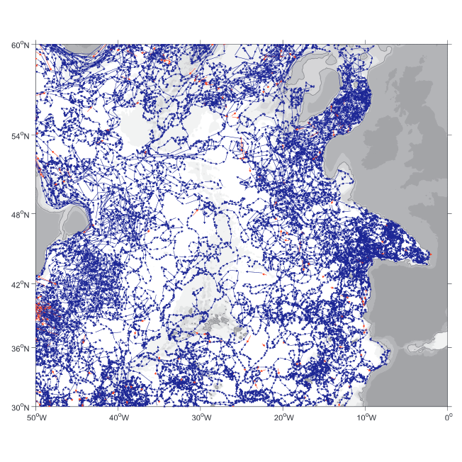
A world deep displacement dataset comprising more than 1600 000 Argo floats deep displacements, has been produced from the global Argo float database (GDAC). ANDRO dataset was completed over the period 2000-2009, then was partially but yearly updated since 2010. ANDRO actual contents and format is described in the user guide, which must be carefully read before using ANDRO (ANDRO format is also described in Ollitrault M. et al (2013)). One important feature of ANDRO is that the pressures measured during float drifts at depth, and suitably averaged are preserved in ANDRO (see Figure 2). To reach this goal, it was necessary to reprocess most of the Argo raw data, because of the many different decoding versions (roughly 100) not always applied by the DACs to the displacement data because they were mainly interested in the p,t,S profiles. The result of our work was the production of comprehensive files, named DEP (for déplacements in French), containing all the possibly retrievable float data. For detailed information and status of the last released ANDRO product, please visit the dedicated Argo France web page: https://www.umr-lops.fr/SNO-Argo/Products/ANDRO-Argo-floats-displacements-Atlas

The ORHAGO campaigns (Observation of the benthic aquatic resources of the Golfe de Gascogne) are designed to collect data on the composition, distribution and change in relative abundance of benthic fish fauna on the continental shelf (depth <100m) in November to December on a yearly basis. The ORHAGO survey was initiated in 2007 with the objective of developing a fishery-independent abundance index for flatfish species, with a particular focus on the common sole (Solea solea) of the Bay of Biscay. In accordance with the ICES-agreed gear for flatfish abundance surveys, ORHAGO employs a 4-meter-beam trawl with a chain mat, 50-millimeter mesh in the net, and 40-millimeter mesh in the cod-end. The sampling plan was designed to ensure full coverage of the common sole habitat in the Bay of Biscay during a period (November-December) for which fish behavior and distribution was suitable for obtaining an unbiased abundance index (young fish move offshore when coastal waters become colder and before the concentrations of the spawning season). The sampling design is a systematic sampling with 49 reference stations. The sampling design was validated in 2013 by the ICES Working Group on Beam Trawl Surveys (WGBEAM). Since 2013, the ORHAGO survey has been used to assess the status of the Bay of Biscay common sole stock (WGBIE, Working Group for the Bay of Biscay and the Iberian Waters Ecoregion).

The main objective of the SWIM Level 2S (L2S) product is to provide along-track directional wave spectra measures, as well as the integrated parameters of the associated wave systems (wave length, significant wave height, direction), over the global ocean, as observed with SWIM instrument onboard CFOSAT. CFOSAT (Chinese French Ocean SATellite) is a french-chinese mission launched in 2018, whose aim is to provide wind (SCAT instrument) and wave (SWIM instrument) measurements over the sea surface. The wave spectra and their associated partitions are provided independently for each SWIM incidence (from 2° to 10°), together with the sigma0 resampled at a 20m resolution. They are complemented with information from the nadir beam such as the sigma0, wind speed, significant wave height or rain flag. The SWIM level 2S (L2S) product is generated in delayed mode, a few days after acquisition. It complements the Near-Real Time (NRT) L2 product delivered by the CWWIC center by providing an alternative and evolutive processing to test and implement quickly new algorithms for the wave inversion over the whole mission archive. These evolutions may take advantage of better ancillary data not available in NRT (ice mask product, best estimates of wind or wave model), of the combination with wind measurements from the onboard SCAT scatterometer. The product is also designed to handle complex situations such as coastal areas and heterogeneous seas. These complex situations are by nature of particular scientific interest (e.g. wind wave interactions, wave evolution in coastal region). This version 2 improves the previous release in particular through a new empirical modulation transfer function (MTF) and better partitioning. The dataset is also lighter in size. It has been completely reprocessed from SWIM Level 1 archive. Note that the dataset is split on the access server in two different sub-versions (**2.0** for the L2S using Level 1 in OP06 version, **2.1** for the L2S using Level 1 in OP07 version). No major differences are expected. The SWIM L2S product is generated and distributed by Ifremer / CERSAT in the frame of the Ifremer Wind and Wave Operation Center (IWWOC) co-funded by Ifremer and CNES and dedicated to the processing of the delayed mode data of CFOSAT mission.

Coastal Surveillance Through Observation of Ocean Color (COASTlOOC) oceanographic expeditions were conducted in 1997 and 1998 to examine the relationship between the optical properties of seawater and related biological and chemical properties across the coastal-to-open ocean gradient in various European seas. A total of 379 stations were visited along the coasts of the Gulf of Lion in the Mediterranean Sea (n = 61), Adriatic Sea (n = 39), Baltic Sea (n = 57), North Sea (n = 99), English Channel (n = 85) and Atlantic Ocean (n = 38). Particular emphasis was dedicated to the collection of a comprehensive set of apparent (AOPs) and inherent (IOPs) optical properties to support the development of ocean color remote sensing algorithms. The data were collected in situ using traditional ship-based sampling, but also from a helicopter, which is a very efficient means for that type of coastal sampling. The dataset collected during the COASTlOOC campaigns is unique in that it is fully consistent in terms of operators, protocols, and instrumentation. This rich and historical dataset is still today frequently requested and used by other researchers. Therefore, we present the result of an effort to compile and standardize a dataset which will facilitate its use in future development and evaluation of new bio-optical models adapted for optically-complex waters.