 Catalogue PIGMA
series
Type of resources
Available actions
Topics
Keywords
Contact for the resource
Provided by
Years
Formats
Representation types
Update frequencies
status
Scale
Resolution
-

Surface current data measured by the CNR-ISMAR HF radar network are made available in graphical format for the last 48 hours and in real time and delayed mode via a THREDDS catalog which provides metadata and data access. The web site gives information on HF radar technology, sites position and operational parameters, and links to the THREDDS catalog. The catalog offers different remote-data-access protocols such as Open-source Project for a Network Data Access Protocol (OpenDaP), Web Coverage Service (WCS), Web Map Service (WMS) (OGS standards), as well as pure HTTP or NetCDF-Subsetter. They allow for metadata interrogation and data download (even sub-setting the dataset in terms of time and space) while embedded clients, such as GODIVA2, NetCDF-JavaToolsUI and Integrated Data Viewer, grant real-time data visualization directly via browser and allow for navigating within the plotted maps, saving images, exporting-importing on Google Earth, generating animations in selected time intervals. The data on the THREDDS catalog are organized in two folders, collecting the hourly current files of the last five days and grouping all the historical data. The two folders are accessible both in aggregated and in non-aggregated configuration. The data set consists of maps of radial and total velocity of the sea water surface current collected by the HF radars within the Italian Coastal Radar Network established in the framework of the Italian flagship project RITMARE. Surface ocean velocities estimated by HF Radar are representative of the upper 0.3-2.5 meters of the ocean. The radar sites are operated according to Quality Assessment procedures and data are processed for Quality Control. Data access tools are compliant to Open Geospatial Consortium (OGC), Climate and Forecast (CF) convention and INSPIRE directive. The use of netCDF format allows an easy implementation of all the open source services developed by UNIDATA.
-
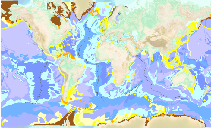
The “World Seabed Sediment Map” product contains geo-referenced digital data, describing the nature of the sediment encountered in different seas and oceans of the world. The objects are all surface areas and the description of an object includes in particular the nature of the sediment including rock-type bottoms.
-
This visualization product displays the cigarette related items abundance of marine macro-litter (> 2.5cm) per beach per year from non-MSFD monitoring surveys, research & cleaning operations without UNEP-MARLIN data. EMODnet Chemistry included the collection of marine litter in its 3rd phase. Since the beginning of 2018, data of beach litter have been gathered and processed in the EMODnet Chemistry Marine Litter Database (MLDB). The harmonization of all the data has been the most challenging task considering the heterogeneity of the data sources, sampling protocols and reference lists used on a European scale. Preliminary processings were necessary to harmonize all the data: - Exclusion of OSPAR 1000 protocol: in order to follow the approach of OSPAR that it is not including these data anymore in the monitoring; - Selection of surveys from non-MSFD monitoring, cleaning and research operations; - Exclusion of beaches without coordinates; - Selection of plastic bags related items only. The list of selected items is attached to this metadata. This list was created using EU Marine Beach Litter Baselines, the European Threshold Value for Macro Litter on Coastlines and the Joint list of litter categories for marine macro-litter monitoring from JRC (these three documents are attached to this metadata); - Exclusion of surveys without associated length; - Normalization of survey lengths to 100m & 1 survey / year: in some case, the survey length was not 100m, so in order to be able to compare the abundance of litter from different beaches a normalization is applied using this formula: Number of plastic bags related items of the survey (normalized by 100 m) = Number of plastic bags related items of the survey x (100 / survey length) Then, this normalized number of plastic bags related items is summed to obtain the total normalized number of plastic bags related items for each survey. Finally, the median abundance of plastic bags related items for each beach and year is calculated from these normalized abundances of plastic bags related items per survey. Percentiles 50, 75, 95 & 99 have been calculated taking into account plastic bags related items from other sources data for all years. More information is available in the attached documents. Warning: the absence of data on the map does not necessarily mean that they do not exist, but that no information has been entered in the Marine Litter Database for this area.
-

"'Short description:''' The High-Resolution Ocean Colour (HR-OC) Consortium (Brockmann Consult, Royal Belgian Institute of Natural Sciences, Flemish Institute for Technological Research) distributes Level 4 (L4) Turbidity (TUR, expressed in FNU), Solid Particulate Matter Concentration (SPM, expressed in mg/l), particulate backscattering at 443nm (BBP443, expressed in m-1) and chlorophyll-a concentration (CHL, expressed in µg/l) for the Sentinel 2/MSI sensor at 100m resolution for a 20km coastal zone. The products are delivered on a geographic lat-lon grid (EPSG:4326). BBP443, constitute the category of the 'optics' products. The BBP443 product is generated from the L3 RRS products using a quasi-analytical algorithm (Lee et al. 2002). he 'tur_tsm_chl' products include TUR, SPM and CHL. They are retrieved through the application of automated switching algorithms to the RRS spectra adapted to varying water conditions (Novoa et al. 2017). The GEOPHYSICAL product consists of the Chlorophyll-a concentration (CHL) retrieved via a multi-algorithm approach with optimized quality flagging (O'Reilly et al. 2019, Gons et al. 2005, Lavigne et al. 2021). Monthly products (P1M) are temporal aggregates of the daily L3 products. Daily products contain gaps in cloudy areas and where there is no overpass at the respective day. Aggregation collects the non-cloudy (and non-frozen) contributions to each pixel. Contributions are averaged per variable. While this does not guarantee data availability in all pixels in case of persistent clouds, it provides a more complete product compared to the sparsely filled daily products. The Monthly L4 products (P1M) are generally provided withing 4 days after the last acquisition date of the month. Daily gap filled L4 products (P1D) are generated using the DINEOF (Data Interpolating Empirical Orthogonal Functions) approach which reconstructs missing data in geophysical datasets by using a truncated Empirical Orthogonal Functions (EOF) basis in an iterative approach. DINEOF reconstructs missing data in a geophysical dataset by extracting the main patterns of temporal and spatial variability from the data. While originally designed for low resolution data products, recent research has resulted in the optimization of DINEOF to handle high resolution data provided by Sentinel-2 MSI, including cloud shadow detection (Alvera-Azcárate et al., 2021). These types of L4 products are generated and delivered one month after the respective period. '''Processing information:''' The HR-OC processing system is deployed on Creodias where Sentinel 2/MSI L1C data are available. The production control element is being hosted within the infrastructure of Brockmann Consult. The processing chain consists of: * Resampling to 60m and mosaic generation of the set of Sentinel-2 MSI L1C granules of a single overpass that cover a single UTM zone. * Application of a glint correction taking into account the detector viewing angles * Application of a coastal mask with 20km water + 20km land. The result is a L1C mosaic tile with data just in the coastal area optimized for compression. * Level 2 processing with pixel identification (IdePix), atmospheric correction (C2RCC and ACOLITE or iCOR), in-water processing and merging (HR-OC L2W processor). The result is a 60m product with the same extent as the L1C mosaic, with variables for optics, transparency, and geophysics, and with data filled in the water part of the coastal area. * invalid pixel identification takes into account corrupted (L1) pixels, clouds, cloud shadow, glint, dry-fallen intertidal flats, coastal mixed-pixels, sea ice, melting ice, floating vegetation, non-water objects, and bottom reflection. * Daily L3 aggregation merges all Level 2 mosaics of a day intersecting with a target tile. All valid water pixels are included in the 20km coastal stripes; all other values are set to NaN. There may be more than a single overpass a day, in particular in the northern regions. This step comprises resampling to the 100m target grid. * Monthly L4 aggregation combines all Level 3 products of a month and a single tile. The output is a set of 3 NetCDF datasets for (1) optics and (2) turbidity, suspended matter and chlorophyll concentration, respectively for the month. * Gap filling combines all daily products of a period and generates (partially) gap-filled daily products again. The output of gap filling are 2 datasets for (1) optics (BBP443 only) and (2) turbidity, suspended mattr and chlorophyll concentration per day. '''Description of observation methods/instruments:''' Ocean colour technique exploits the emerging electromagnetic radiation from the sea surface in different wavelengths. The spectral variability of this signal defines the so-called ocean colour which is affected by the presence of phytoplankton. '''Quality / Accuracy / Calibration information:''' A detailed description of the calibration and validation activities performed over this product can be found on the CMEMS web portal and in CMEMS-BGP_HR-QUID-009-201_to_212. '''Suitability, Expected type of users / uses:''' This product is meant for use for educational purposes and for the managing of the marine safety, marine resources, marine and coastal environment and for climate and seasonal studies. '''Dataset names: ''' *cmems_obs_oc_med_bgc_tur_spm_chl_nrt_l4-hr-mosaic_P1M-v01 *cmems_obs_oc_med_bgc_optics_nrt_l4-hr-mosaic_P1M-v01 *cmems_obs_oc_med_bgc_tur_spm_chl_nrt_l4-hr-mosaic_P1D-v01 *cmems_obs_oc_med_bgc_optics_nrt_l4-hr-mosaic_P1D-v01 '''Files format:''' *netCDF-4, CF-1.7 *INSPIRE compliant." '''DOI (product) :''' https://doi.org/10.48670/moi-00110
-
-

'''Short description:''' These products integrate wave observations aggregated and validated from the Regional EuroGOOS consortium (Arctic-ROOS, BOOS, NOOS, IBI-ROOS, MONGOOS) and Black Sea GOOS as well as from National Data Centers (NODCs) and JCOMM global systems (OceanSITES, DBCP) and the Global telecommunication system (GTS) used by the Met Offices. '''DOI (product) :''' https://doi.org/10.17882/70345
-
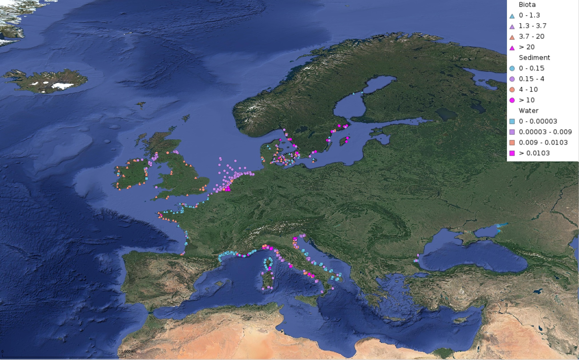
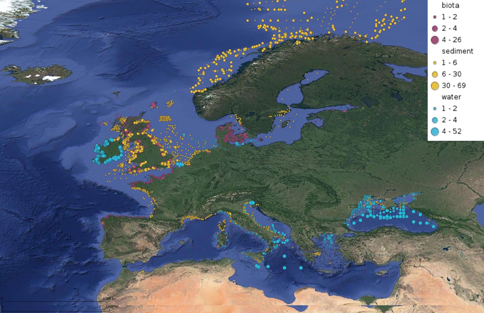
This product displays for Tributyltin, median values of the last 6 available years that have been measured per matrix and are present in EMODnet regional contaminants aggregated datasets, v2022. The median values ranges are derived from the following percentiles: 0-25%, 25-75%, 75-90%, >90%. Only "good data" are used, namely data with Quality Flag=1, 2, 6, Q (SeaDataNet Quality Flag schema). For water, only surface values are used (0-15 m), for sediment and biota data at all depths are used.
-
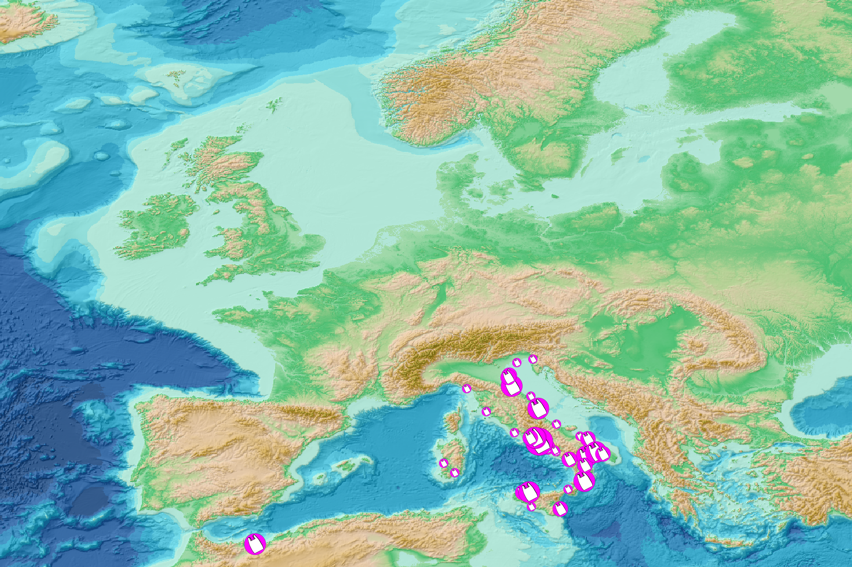
This product displays for Benzo(a)pyrene, positions with values counts that have been measured per matrix for each year and are present in EMODnet regional contaminants aggregated datasets, v2022. The product displays positions for every available year.
-

GO-SHIP, the Global Ocean Ship-Based Hydrographic Investigations Program, is conducting repeat hydrography with high accuracy high precision reference measurements of a variety of EOVs through the whole water column. A selection of continent-to-continent full depth sections are repeated at roughly decadal intervals. The data archive for CTD data and bottle data is currently at CCHDO, although the CTD data from European cruises are available at Seadatanet as well.
-
Bathymetric datasets are an extraction of surveys belonging to the Shom public database. For depth up to 50m, the vertical precision of soundings varies from 30cm to 1m and the horizontal precision varies from 1 to 20m. In deep ocean, the vertical precision is mainly around 1 or 2% of the bottom depth. It is sometimes more, it depends on the technology used. The data are referenced to ZH which is assimilated to LAT. Data are corrected for sound velocity variations. <br /> October 27 2025 version