List of fish stocks referenced for the year 2018. The repository includes 477 stocks. Each stock is identified by a unique key in accordance with the ICES codification in use. Each record contains a stock identifier, a species or group of species identifier according to the ASFIS/FAO classification, the English stock name, the Latin name of the species, the assessment area according to the FAO codification of fishing sectors. When the stock assessment area groups a series of sectors, the first and last sectors in the series are separated by a dash.

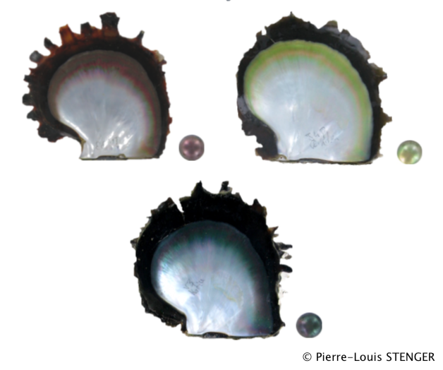
Whole genome pooled sequencing of individuals from 4 populations and 3 different color phenotype in order to uncover the genetic variants linked to color expression in the pearl oyster P. margaritifera.

Rapport final ONF

The All-Atlantic Ocean Research and Innovation Alliance (AAORIA) is the result of science diplomacy efforts involving countries from both sides of the Atlantic Ocean. It builds upon the success of two existing cooperative agreements – the Galway Statement on Atlantic Ocean Cooperation which was signed by the European Union, United States, and Canada in 2013; and the Belem Statement on Atlantic Ocean Research and Innovation Cooperation which was signed by the European Union, Brazil, and South Africa in 2017 as well as on several other bilateral and multilateral agreements. AAORIA aims to enhance marine research and innovation cooperation along and across the Atlantic Ocean. In 2022, the “All-Atlantic Declaration” was signed to revitalize collaboration among current initiatives and enhance the coordination between the Galway Working Groups, All-Atlantic Joint Pilot Actions, and related projects. Additionally, it aims to engage new partners and initiatives to join the All-Atlantic community.

'''DEFINITION''' The time series are derived from the regional chlorophyll reprocessed (MY) product as distributed by CMEMS (OCEANCOLOUR_MED_BGC_L3_NRT_009_141). This dataset, derived from multi-sensor (SeaStar-SeaWiFS, AQUA-MODIS, NOAA20-VIIRS, NPP-VIIRS, Envisat-MERIS and Sentinel3-OLCI) Rrs spectra produced by CNR using an in-house processing chain, is obtained by means of the Mediterranean Ocean Colour regional algorithms: an updated version of the MedOC4 (Case 1 (off-shore) waters, Volpe et al., 2019, with new coefficients) and AD4 (Case 2 (coastal) waters, Berthon and Zibordi, 2004). The processing chain and the techniques used for algorithms merging are detailed in Colella et al. (2023). Monthly regional mean values are calculated by performing the average of 2D monthly mean (weighted by pixel area) over the region of interest. The deseasonalized time series is obtained by applying the X-11 seasonal adjustment methodology on the original time series as described in Colella et al. (2016), and then the Mann-Kendall test (Mann, 1945; Kendall, 1975) and Sens’s method (Sen, 1968) are subsequently applied to obtain the magnitude of trend. This OMI has been introduced since the 2nd issue of Ocean State Report in 2017. '''CONTEXT''' Phytoplankton and chlorophyll concentration as a proxy for phytoplankton respond rapidly to changes in environmental conditions, such as light, temperature, nutrients and mixing (Colella et al. 2016). The character of the response depends on the nature of the change drivers, and ranges from seasonal cycles to decadal oscillations (Basterretxea et al. 2018). Therefore, it is of critical importance to monitor chlorophyll concentration at multiple temporal and spatial scales, in order to be able to separate potential long-term climate signals from natural variability in the short term. In particular, phytoplankton in the Mediterranean Sea is known to respond to climate variability associated with the North Atlantic Oscillation (NAO) and El Niño Southern Oscillation (ENSO) (Basterretxea et al. 2018, Colella et al. 2016). '''KEY FINDINGS''' In the Mediterranean Sea, the average chlorophyll trend for the 1997–2024 period is slightly negative, at -0.77 ± 0.59% per year, reinforcing the findings of the previous releases. This result contrasts with the analysis by Sathyendranath et al. (2018), which reported increasing chlorophyll concentrations across all European seas. From around 2010–2011 onward, excluding the 2018–2019 period, a noticeable decline in chlorophyll levels is evident in the deseasonalized time series (green line) and in the observed maxima (grey line), particularly from 2015. This sustained decline over the past decade contributes to the overall negative trend observed in the Mediterranean Sea. '''DOI (product):''' https://doi.org/10.48670/moi-00259

Tronçons linéaires de voies de l'Aquitaine romaine - projet Aquitaviae

'''DEFINITION''' The trend map is derived from version 5 of the global climate-quality chlorophyll time series produced by the ESA Ocean Colour Climate Change Initiative (ESA OC-CCI, Sathyendranath et al. 2019; Jackson 2020) and distributed by CMEMS. The trend detection method is based on the Census-I algorithm as described by Vantrepotte et al. (2009), where the time series is decomposed as a fixed seasonal cycle plus a linear trend component plus a residual component. The linear trend is expressed in % year -1, and its level of significance (p) calculated using a t-test. Only significant trends (p < 0.05) are included. '''CONTEXT''' Phytoplankton are key actors in the carbon cycle and, as such, recognised as an Essential Climate Variable (ECV). Chlorophyll concentration is the most widely used measure of the concentration of phytoplankton present in the ocean. Drivers for chlorophyll variability range from small-scale seasonal cycles to long-term climate oscillations and, most importantly, anthropogenic climate change. Due to such diverse factors, the detection of climate signals requires a long-term time series of consistent, well-calibrated, climate-quality data record. Furthermore, chlorophyll analysis also demands the use of robust statistical temporal decomposition techniques, in order to separate the long-term signal from the seasonal component of the time series. '''CMEMS KEY FINDINGS''' The average global trend for the 1997-2021 period was 0.51% per year, with a maximum value of 25% per year and a minimum value of -6.1% per year. Positive trends are pronounced in the high latitudes of both northern and southern hemispheres. The significant increases in chlorophyll reported in 2016-2017 (Sathyendranath et al., 2018b) for the Atlantic and Pacific oceans at high latitudes appear to be plateauing after the 2021 extension. The negative trends shown in equatorial waters in 2020 appear to be remain consistent in 2021. '''DOI (product):''' https://doi.org/10.48670/moi-00230

Annual time series of salmon escapement (2009-2014): • Time series of atlantic salmon escapement • Location and Long Term Average (LTA) of atlantic salmon escapement per Management Unit, that could be a river, basin district, a region or a whole country.

Phyto plankton Abundance: Identify the 3 most abundant phytoplankton species in the North Atlantic and calculate a timeseries of their abundance within the basin.

North Atlantic basin average at Pentadal (5-year) resolution time-series of the ocean heat storage (upper 700m) and kinetic energy. Use gridded information to calculate the local heat storage and average kinetic energy as a 5 year average and then calculate the basin average.