 Catalogue PIGMA
2023
Type of resources
Available actions
Topics
Keywords
Contact for the resource
Provided by
Years
Formats
Representation types
Update frequencies
status
Scale
Resolution
-

Comparison between 3 kits, Roche, Twist Biosciences and Illumina on the ability to enrich environmental samples to viral sequences
-

Species distribution models (Random Forest) predicting the distribution of mixed cold-water coral community (Coral Garden) assemblage in the Celtic Sea. This community is considered ecologically coherent according to the cluster analysis conducted by Parry et al. (2015) on image sample. Modelling its distribution complements existing work on their definition and offers a representation of the extent of the areas of the North East Atlantic where they can occur based on the best available knowledge. This work was performed at the University of Plymouth in 2021.
-

Classification of the Atlantic Ocean seabed into broad-scale benthic habitats employing a hierarchical top-down clustering approach aimed at informing Marine Spatial Planning. This work was performed at the University of Plymouth in 2021 with data provided by a wide group of partners representing the nations surrounding the Atlantic Ocean. It classifies continuous environmental data into discrete classes that can be compared to observed biogeographical patterns at various scales. It has 3 levels of classification. For ease of use, a layer is provided for each level. Level 1 has 4 classes. Level 2 has 15 classes nested within level 1. Layers indices are 2 digits (1[level1 class index]1[level 2 class index]). Level 3 has 157 classes nested within level 2 and class names have 4 digits (1digit[level1 class index]1[level 2 class index]2[level 3 class index]). Note that the classification was performed for the whole world and thus it has more classes than in the presented layer.
-

Classification of the seabed in the Atlantic Ocean into broad-scale benthic habitats employing a non-hierarchical top-down clustering approach aimed at informing Marine Spatial Planning. This work was performed at the University of Plymouth in 2021 with data provided by a wide group of partners representing the nations surrounding the Atlantic Ocean. It classifies continuous environmental data into discrete classes that can be compared to observed biogeographical patterns at various scales. It has 3 levels of classification. The numbers in the raster layer correspond to individual classes. Description of these classes is given in McQuaid, K.A. et al. (2023).
-
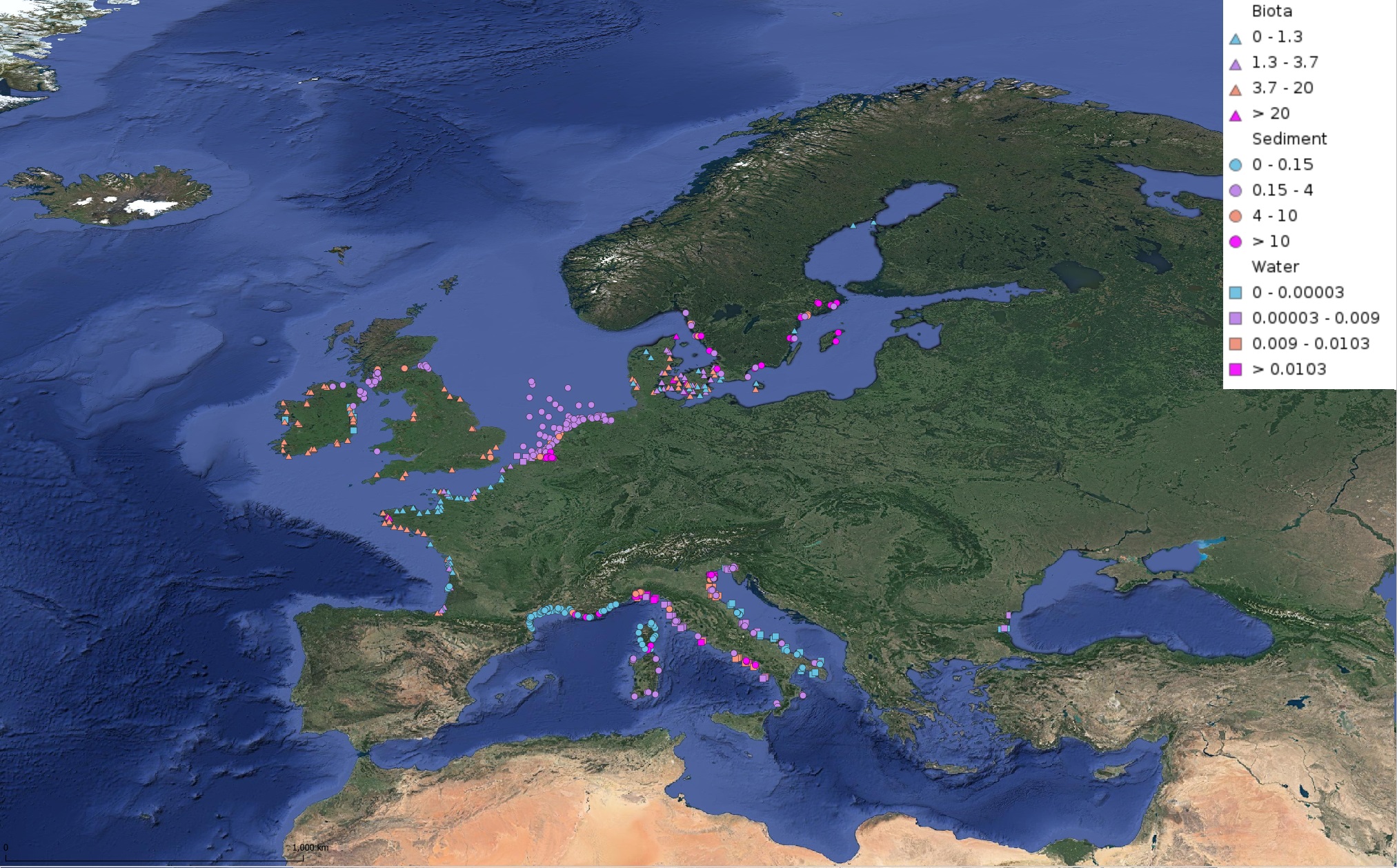
This product displays for Tributyltin, median values of the last 6 available years that have been measured per matrix and are present in EMODnet regional contaminants aggregated datasets, v2022. The median values ranges are derived from the following percentiles: 0-25%, 25-75%, 75-90%, >90%. Only "good data" are used, namely data with Quality Flag=1, 2, 6, Q (SeaDataNet Quality Flag schema). For water, only surface values are used (0-15 m), for sediment and biota data at all depths are used.
-
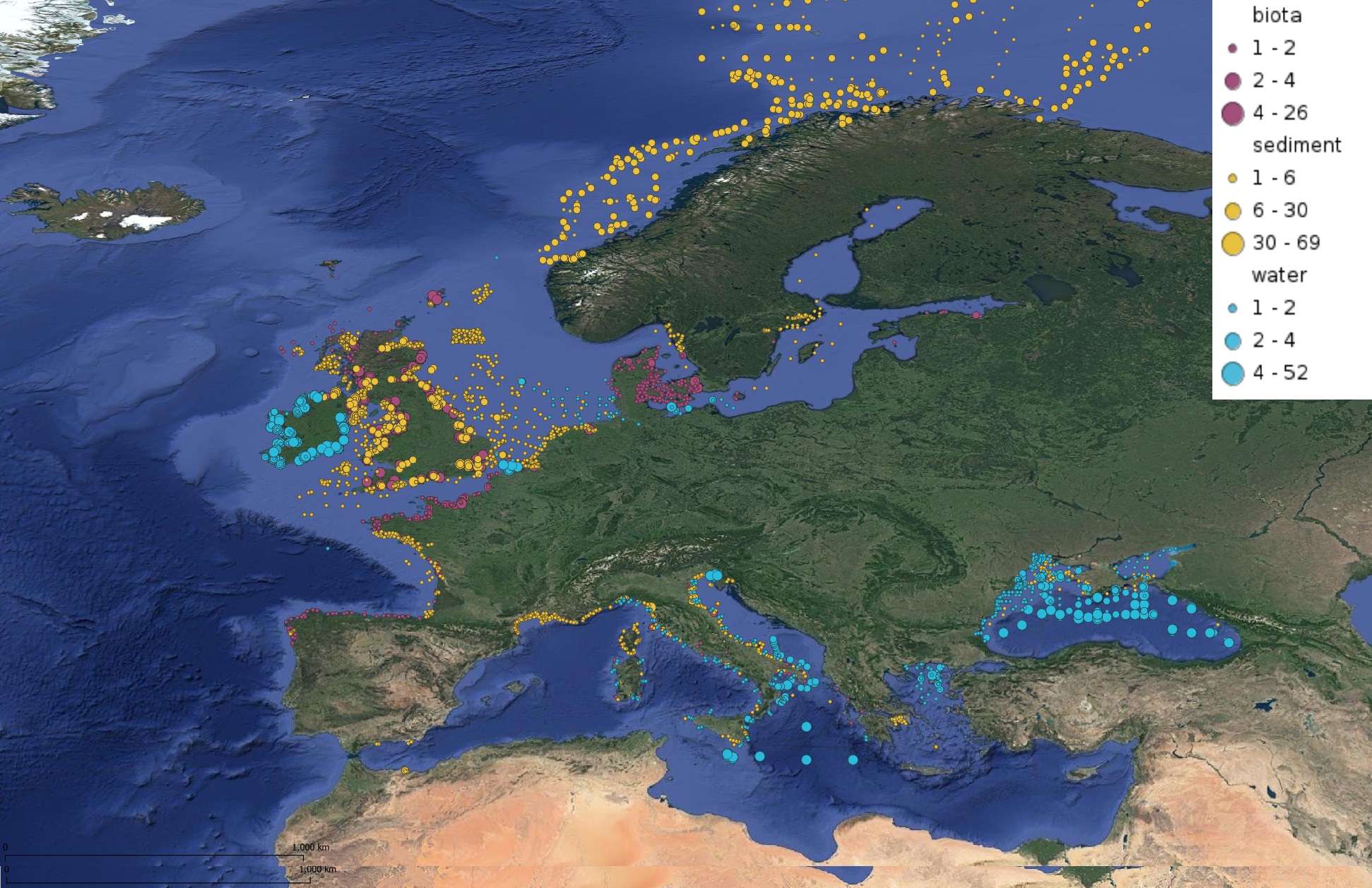
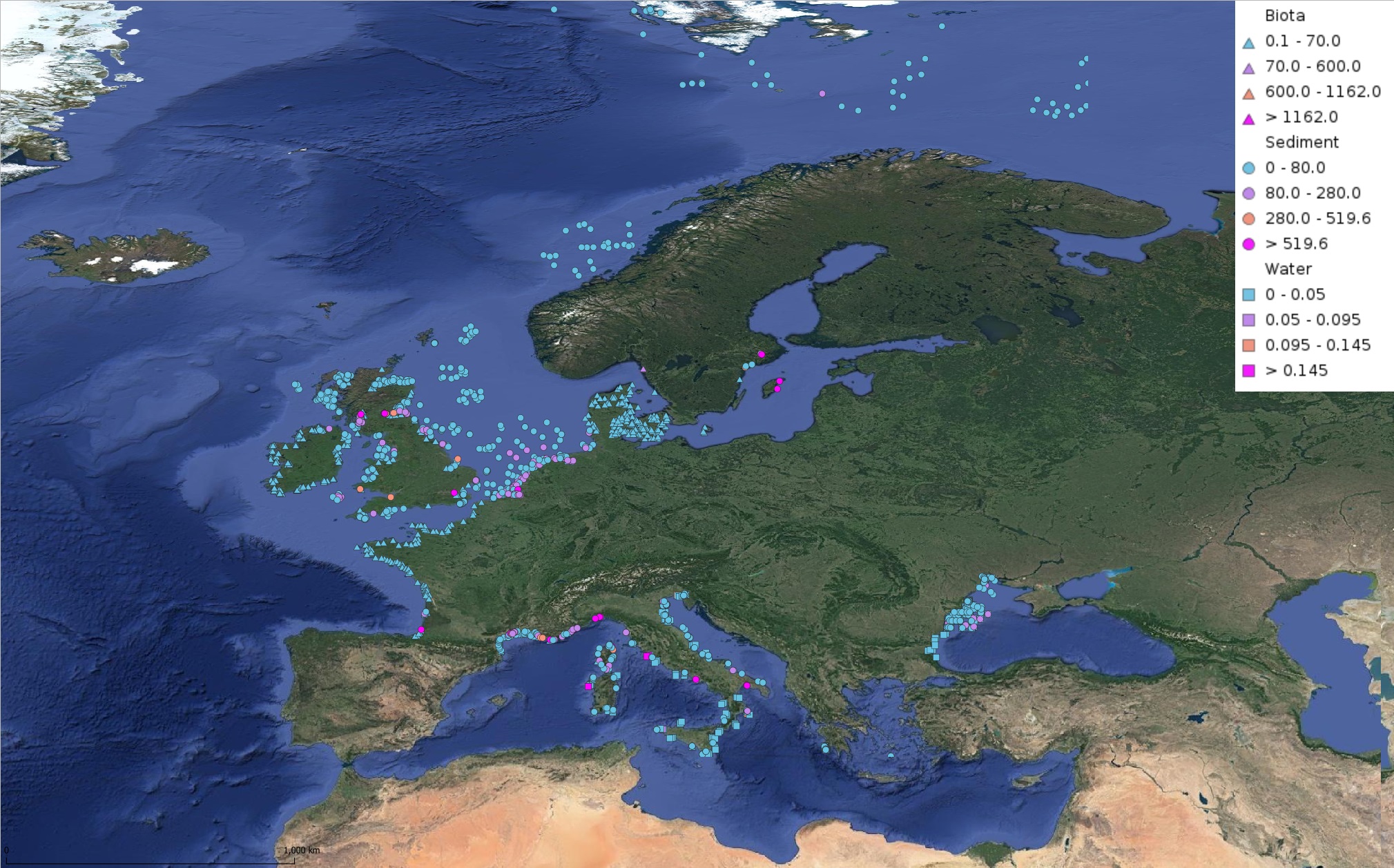
This product displays for Benzo(a)pyrene, positions with values counts that have been measured per matrix for each year and are present in EMODnet regional contaminants aggregated datasets, v2022. The product displays positions for every available year.
-
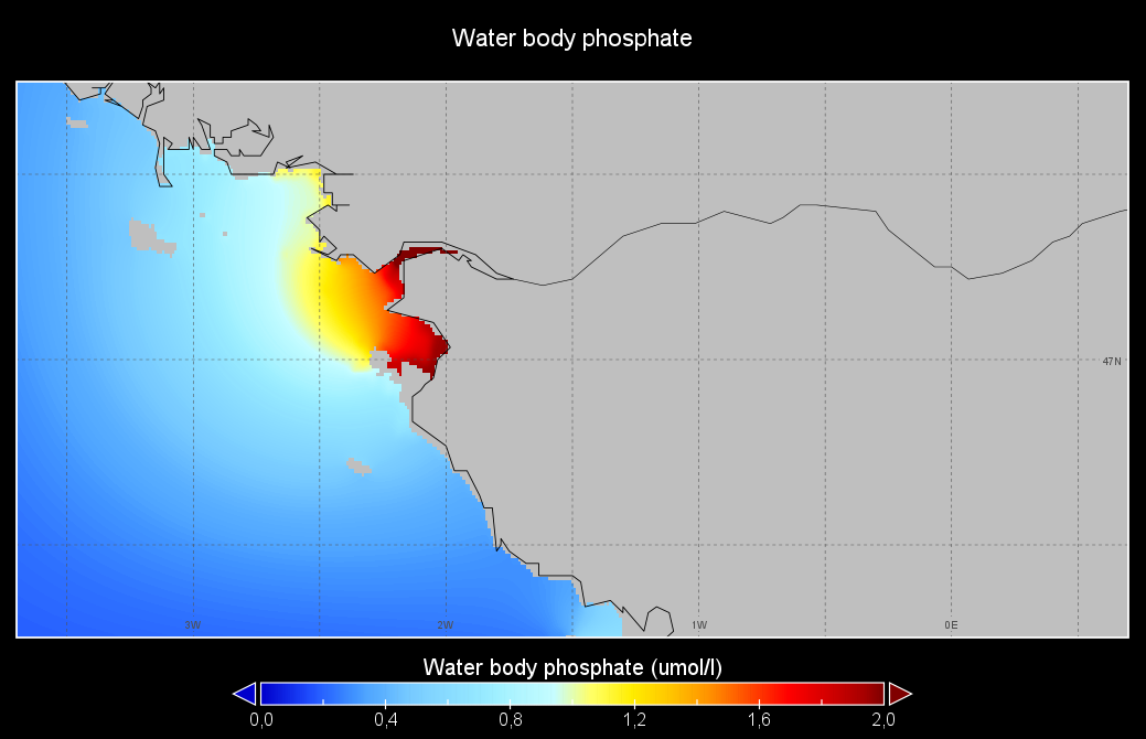
Seasonal climatology of Water body phosphate for Loire river for the period 1950-2021 and for the following seasons: - winter: January-March, - spring: April-June, - summer: July-September, - autumn: October-December. Observation data span from 1950 to 2021. Depth levels (m): [0.0, 2.0, 4.0, 6.0, 8.0, 10.0, 15.0, 20.0, 25.0, 30.0, 35.0, 40.0, 45.0, 50.0, 60.0, 70.0, 80.0, 90.0, 100.0, 110.0, 120.0, 130.0]. Data sources: observational data from SeaDataNet/EMODNet Chemistry Data Network. Description of DIVAnd analysis: the computation was done with DIVAnd (Data-Interpolating Variational Analysis in n dimensions), version 2.7.4, using GEBCO 15 sec topography for the spatial connectivity of water masses. The horizontal resolution of the produced DIVAnd maps is 0.01 degrees. Horizontal correlation length is defined seasonally (in meters): 230000 (winter), 264000 (spring), 140000 (summer), 135000 (autumn). Vertical correlation length was optimized and vertically filtered and a seasonally-averaged profile was used (DIVAnd.fitvertlen). Signal-to-noise ratio was fixed to 1 for vertical profiles and 0.1 for time series to account for the redundancy in the time series observations. A logarithmic transformation (DIVAnd.Anam.loglin) was applied to the data prior to the analysis to avoid unrealistic negative values. Background field: the vertically-filtered data mean profile is substracted from the data. Detrending of data: no, advection constraint applied: no. Units: umol/l.
-
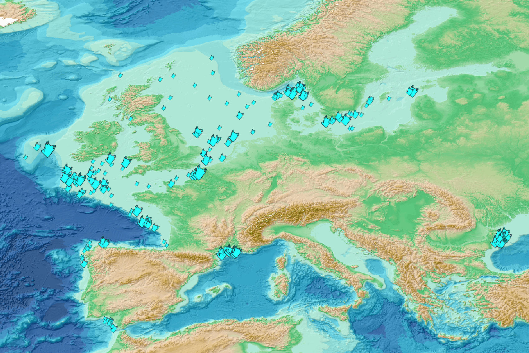
This visualization product displays plastic bags density per trawl. EMODnet Chemistry included the collection of marine litter in its 3rd phase. Since the beginning of 2018, data of seafloor litter collected by international fish-trawl surveys have been gathered and processed in the EMODnet Chemistry Marine Litter Database (MLDB). The harmonization of all the data has been the most challenging task considering the heterogeneity of the data sources, sampling protocols (OSPAR and MEDITS protocols) and reference lists used on a European scale. Moreover, within the same protocol, different gear types are deployed during fishing bottom trawl surveys. In cases where the wingspread and/or number of items were unknown, data could not be used because these fields are needed to calculate the density. Data collected before 2011 are affected by this filter. When the distance reported in the data was null, it was calculated from: - the ground speed and the haul duration using this formula: Distance (km) = Haul duration (h) * Ground speed (km/h); - the trawl coordinates if the ground speed and the haul duration were not filled in. The swept area is calculated from the wingspread (which depends on the fishing gear type) and the distance trawled: Swept area (km²) = Distance (km) * Wingspread (km) Densities have been calculated on each trawl and year using the following computation: Density of plastic bags (number of items per km²) = ∑Number of plastic bags related items / Swept area (km²) Percentiles 50, 75, 95 & 99 have been calculated taking into account data for all years. The list of selected items for this product is attached to this metadata. Information on data processing and calculation is detailed in the attached methodology document. Warning: the absence of data on the map doesn't necessarily mean that they don't exist, but that no information has been entered in the Marine Litter Database for this area.
-
This product displays for Fluoranthene, median values of the last 6 available years that have been measured per matrix and are present in EMODnet regional contaminants aggregated datasets, v2022. The median values ranges are derived from the following percentiles: 0-25%, 25-75%, 75-90%, >90%. Only "good data" are used, namely data with Quality Flag=1, 2, 6, Q (SeaDataNet Quality Flag schema). For water, only surface values are used (0-15 m), for sediment and biota data at all depths are used.
-

This product displays for Nickel, positions with percentages of all available data values per group of animals that are present in EMODnet regional contaminants aggregated datasets, v2022. The product displays positions for all available years.