 Catalogue PIGMA
2021
Type of resources
Available actions
Topics
Keywords
Contact for the resource
Provided by
Years
Formats
Representation types
Update frequencies
status
Scale
Resolution
-
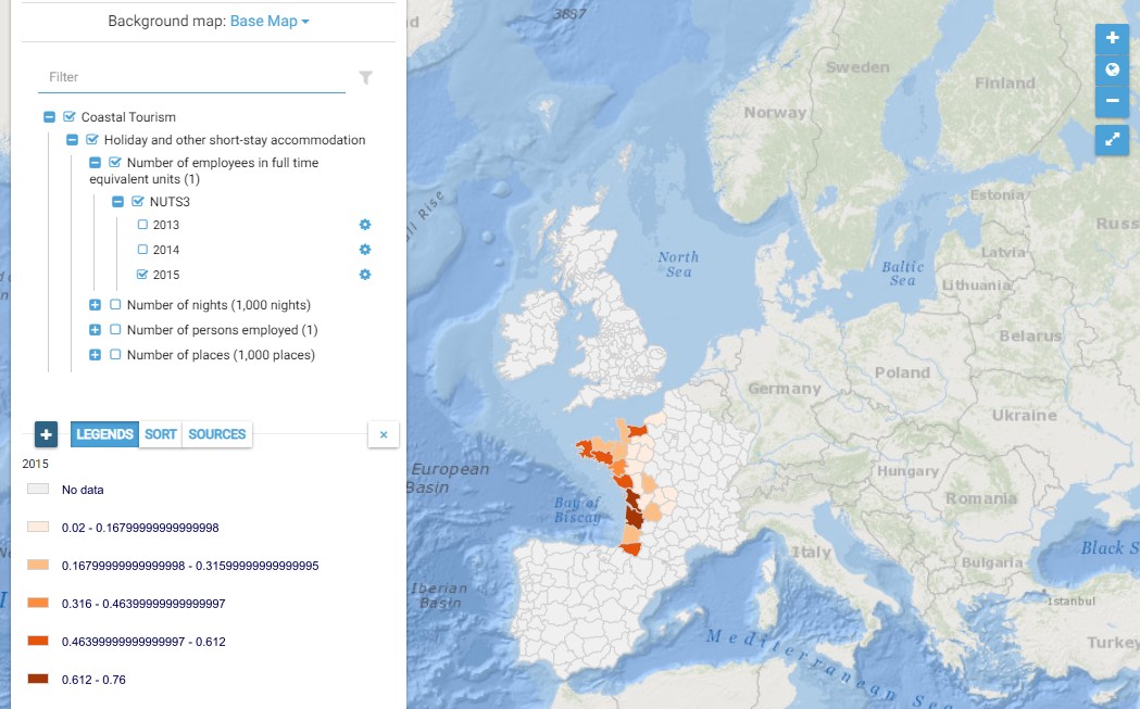
This map presents all layers corresponding to "Holiday and other short-stay accommodation" activities in the Atlantic area. For more information about this NACE code : https://ec.europa.eu/eurostat/ramon/nomenclatures/index.cfm?TargetUrl=DSP_NOM_DTL_VIEW&StrNom=NACE_REV2&StrLanguageCode=EN&IntPcKey=18513794&IntKey=18513824&StrLayoutCode=HIERARCHIC&IntCurrentPage=1 Indicators collected are : Number of places per NUTS 3 unit of the Atlantic Area
-
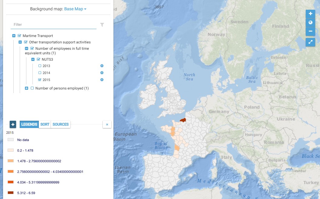
This map presents all layers corresponding to "Other transportation support activities" activities in the Atlantic area. For more information about this NACE code : https://ec.europa.eu/eurostat/ramon/nomenclatures/index.cfm?TargetUrl=DSP_NOM_DTL_VIEW&StrNom=NACE_REV2&StrLanguageCode=EN&IntPcKey=18513344&IntKey=18513494&StrLayoutCode=HIERARCHIC&IntCurrentPage=1 Indicators collected are : Number of persons employed and number of employees in full time equivalent units per NUTS 3 unit of the Atlantic Area
-
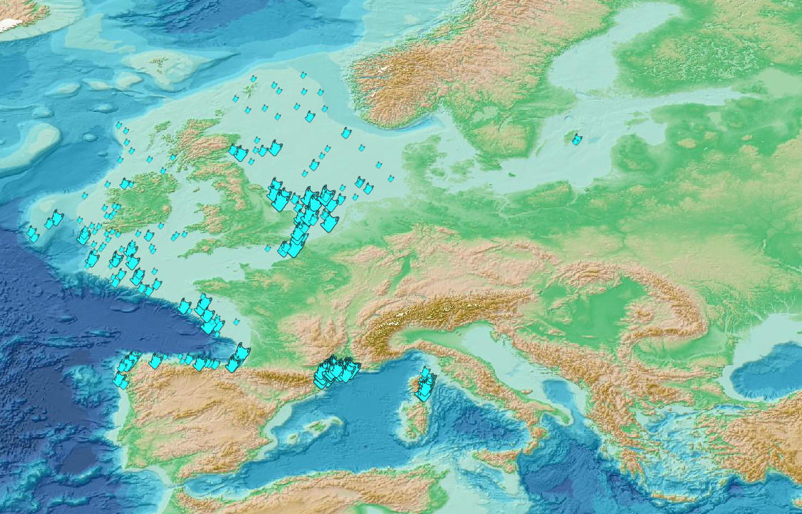
This visualization product displays plastic bags density per trawl. EMODnet Chemistry included the collection of marine litter in its 3rd phase. Since the beginning of 2018, data of seafloor litter collected by international fish-trawl surveys have been gathered and processed in the EMODnet Chemistry Marine Litter Database (MLDB). The harmonization of all the data has been the most challenging task considering the heterogeneity of the data sources, sampling protocols (OSPAR and MEDITS protocols) and reference lists used on a European scale. Moreover, within the same protocol, different gear types are deployed during fishing bottom trawl surveys. In cases where the wingspread and/or number of items were unknown, data could not be used because these fields are needed to calculate the density. Data collected before 2011 are affected by this filter. When the distance reported in the data was null, it was calculated from: - the ground speed and the haul duration using this formula: Distance (km) = Haul duration (h) * Ground speed (km/h); - the trawl coordinates if the ground speed and the haul duration were not filled in. The swept area is calculated from the wingspread (which depends on the fishing gear type) and the distance trawled: Swept area (km²) = Distance (km) * Wingspread (km) Densities have been calculated on each trawl and year using the following computation: Density of plastic bags (number of items per km²) = ∑Number of plastic bags related items / Swept area (km²) Percentiles 50, 75, 95 & 99 have been calculated taking into account data for all years. The list of selected items for this product is attached to this metadata. Information on data processing and calculation is detailed in the attached methodology document. Warning: the absence of data on the map doesn't necessarily mean that they don't exist, but that no information has been entered in the Marine Litter Database for this area.
-
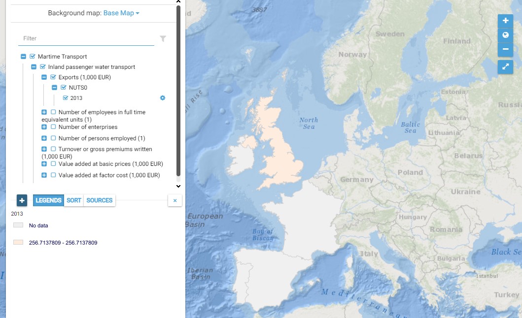
This map presents all layers corresponding to "Inland passenger water transport" activities in the Atlantic area. For more information about this NACE code : https://ec.europa.eu/eurostat/ramon/nomenclatures/index.cfm?TargetUrl=DSP_NOM_DTL_VIEW&StrNom=NACE_REV2&StrLanguageCode=EN&IntPcKey=18512804&IntKey=18512954&StrLayoutCode=HIERARCHIC&IntCurrentPage=1 Indicators collected are : Business indicators per country
-
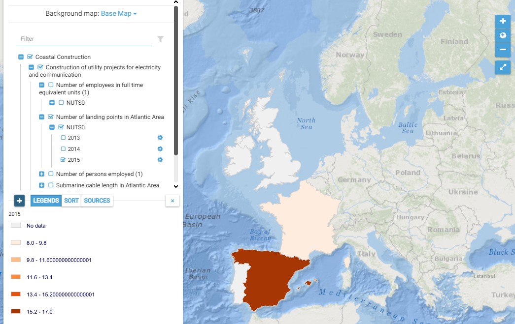
This map presents all layers corresponding to "Construction of utility projects for electricity and communication" activities in the Atlantic area. For more information about this NACE code : https://ec.europa.eu/eurostat/ramon/nomenclatures/index.cfm?TargetUrl=DSP_NOM_DTL_VIEW&StrNom=NACE_REV2&StrLanguageCode=EN&IntPcKey=18508154&IntKey=18508214&StrLayoutCode=HIERARCHIC&IntCurrentPage=1 Indicators collected are : Number of persons employed in cable and pipe laying and maintenance activities in the Atlantic area per country Submarine pipe length in Atlantic Area per country (P16) Number of landing points in Atlantic Area per country
-
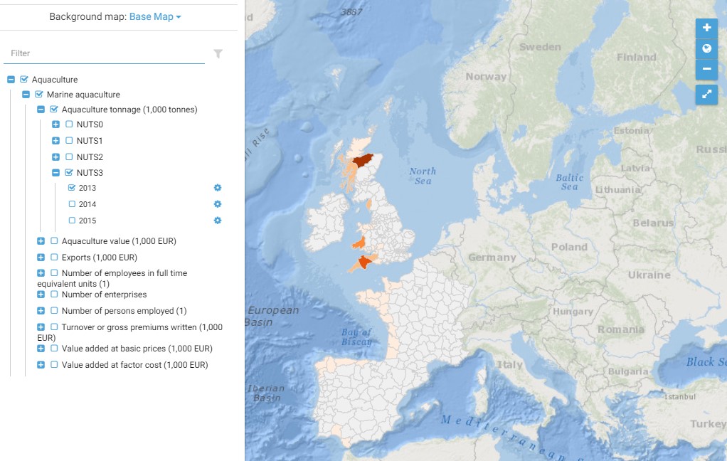
This map presents all layers corresponding to "Marine aquculture" activities in the Atlantic area. For more information about this NACE code : https://ec.europa.eu/eurostat/ramon/nomenclatures/index.cfm?TargetUrl=DSP_NOM_DTL_VIEW&StrNom=NACE_REV2&StrLanguageCode=FR&IntPcKey=18495314&IntKey=18495344&StrLayoutCode=HIERARCHIC&IntCurrentPage=1 Indicators collected are : - Business indicators per country - Number of persons employed and number of employees in full time equivalent units per NUTS 3 unit of the Atlantic Area - Tonnage produced per Atlantic NUTS3 unit - Value produced per Atlantic NUTS 3 unit
-
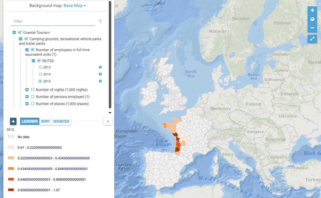
This map presents all layers corresponding to "Camping grounds, recreational vehicle parks and trailer parks" activities in the Atlantic area. For more information about this NACE code : https://ec.europa.eu/eurostat/ramon/nomenclatures/index.cfm?TargetUrl=DSP_NOM_DTL_VIEW&StrNom=NACE_REV2&StrLanguageCode=EN&IntPcKey=18513734&IntKey=18513764&StrLayoutCode=HIERARCHIC&IntCurrentPage=1 Indicators collected are : Number of places per NUTS 3 unit of the Atlantic Area
-
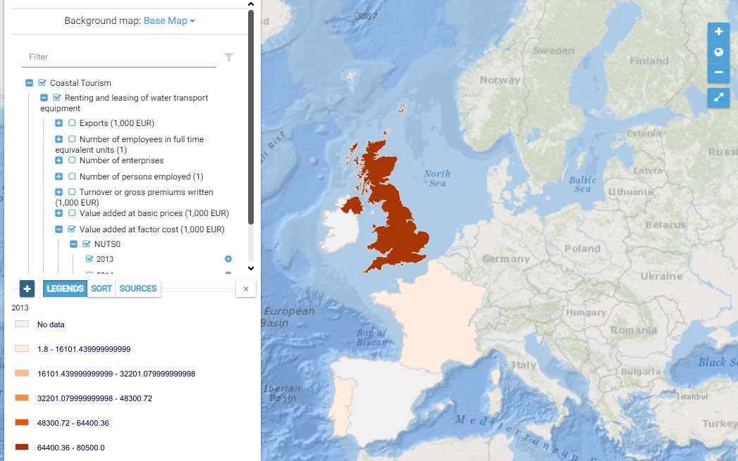
This map presents all layers corresponding to "Renting and leasing of water transport equipment" activities in the Atlantic area. For more information about this NACE code : https://ec.europa.eu/eurostat/ramon/nomenclatures/index.cfm?TargetUrl=DSP_NOM_DTL_VIEW&StrNom=NACE_REV2&StrLanguageCode=EN&IntPcKey=18518354&IntKey=18518474&StrLayoutCode=HIERARCHIC&IntCurrentPage=1 Indicators collected are : Business indicators per country Number of persons employed and number of employees in full time equivalent units per NUTS 3 unit of the Atlantic Area
-
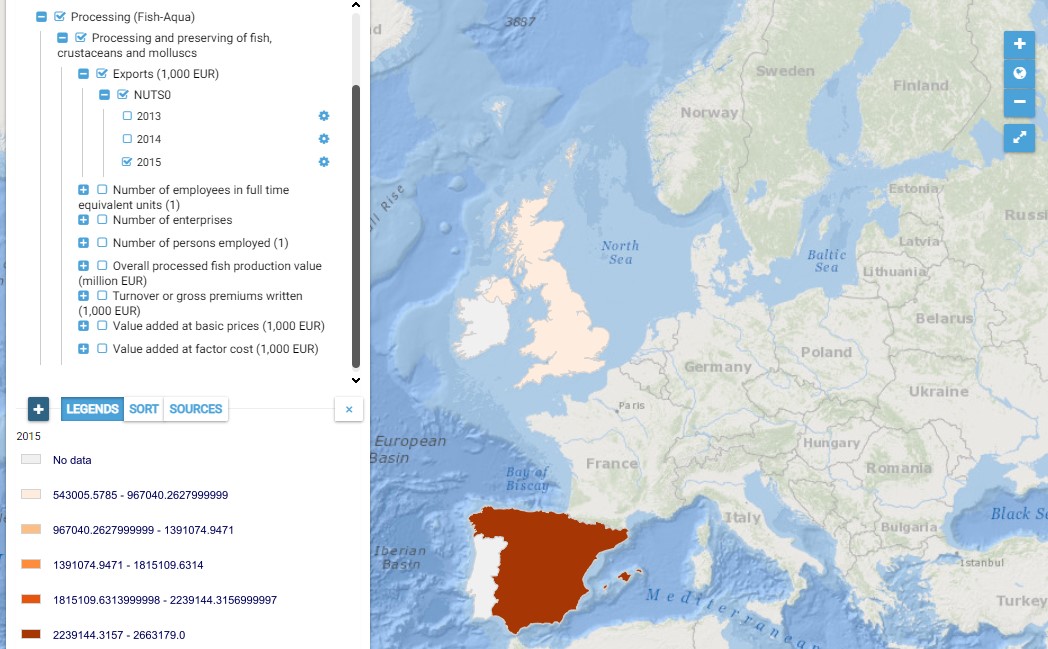
This map presents all layers corresponding to "Processing and preserving of fish, crustaceans and molluscs" activities in the Atlantic area. For more information about this NACE code : https://ec.europa.eu/eurostat/ramon/nomenclatures/index.cfm?TargetUrl=DSP_NOM_DTL_VIEW&StrNom=NACE_REV2&StrLanguageCode=EN&IntPcKey=18496514&IntKey=18496544&StrLayoutCode=HIERARCHIC&IntCurrentPage=1 Indicators collected are : Business indicators per country Total number of persons employed per Atlantic NUTS 3 unit Total production value in the Atlantic NUTS 3 units.
-
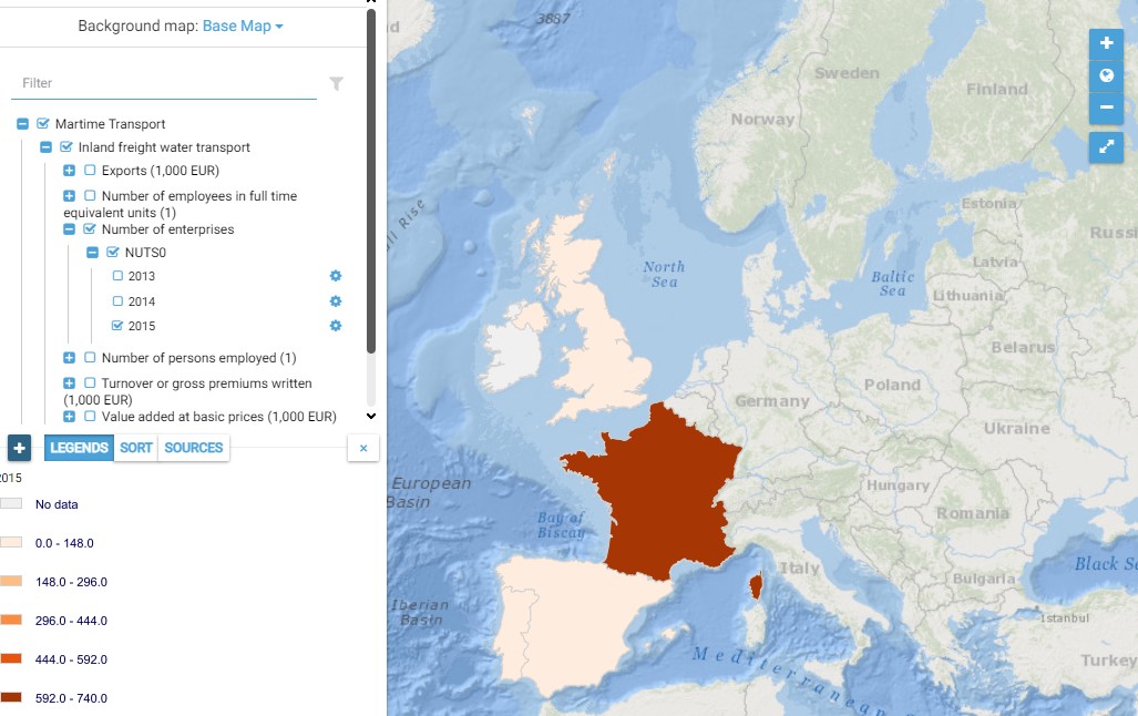
This map presents all layers corresponding to "Inland freight water transport" activities in the Atlantic area. For more information about this NACE code : https://ec.europa.eu/eurostat/ramon/nomenclatures/index.cfm?TargetUrl=DSP_NOM_DTL_VIEW&StrNom=NACE_REV2&StrLanguageCode=EN&IntPcKey=18512804&IntKey=18513014&StrLayoutCode=HIERARCHIC&IntCurrentPage=1 Indicators collected are : Business indicators per country