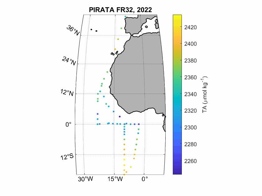
Seawater samples (500 mL) were taken during the PIRATA FR-32 cruise to measure surface inorganic carbon and alkalinity. The analyses were realised by potentiometric titration using a closed-cell at the SNAPO-CO2, LOCEAN in Paris.

'''DEFINITION''' The omi_climate_sst_ibi_trend product includes the Sea Surface Temperature (SST) trend for the Iberia-Biscay-Irish areas over the period 1982-2024, i.e. the rate of change (°C/year). This OMI is derived from the CMEMS REP ATL L4 SST product (SST_ATL_SST_L4_REP_OBSERVATIONS_010_026), see e.g. the OMI QUID, http://marine.copernicus.eu/documents/QUID/CMEMS-OMI-QUID-CLIMATE-SST-IBI_v3.pdf), which provided the SSTs used to compute the SST trend over the Iberia-Biscay-Irish areas. This reprocessed product consists of daily (nighttime) interpolated 0.05° grid resolution SST maps built from re-processed ESA SST CCI, C3S (Embury et al., 2024). Trend analysis has been performed by using the X-11 seasonal adjustment procedure (see e.g. Pezzulli et al., 2005), which has the effect of filtering the input SST time series acting as a low bandpass filter for interannual variations. Mann-Kendall test and Sens’s method (Sen 1968) were applied to assess whether there was a monotonic upward or downward trend and to estimate the slope of the trend and its 95% confidence interval. The reference for this OMI can be found in the first and second issue of the Copernicus Marine Service Ocean State Report (OSR), Section 1.1 (Roquet et al., 2016; Mulet et al., 2018). '''CONTEXT''' Sea surface temperature (SST) is a key climate variable since it deeply contributes in regulating climate and its variability (Deser et al., 2010). SST is then essential to monitor and characterise the state of the global climate system (GCOS 2010). Long-term SST variability, from interannual to (multi-)decadal timescales, provides insight into the slow variations/changes in SST, i.e. the temperature trend (e.g., Pezzulli et al., 2005). In addition, on shorter timescales, SST anomalies become an essential indicator for extreme events, as e.g. marine heatwaves (Hobday et al., 2018). '''CMEMS KEY FINDINGS''' The overall trend in the SST anomalies in this region is 0.012 ±0.001 °C/year over the period 1982-2024. '''DOI (product):''' https://doi.org/10.48670/moi-00257

This visualization product displays the fishing & aquaculture related plastic items abundance of marine macro-litter (> 2.5cm) per beach per year from non-MSFD monitoring surveys, research & cleaning operations. EMODnet Chemistry included the collection of marine litter in its 3rd phase. Since the beginning of 2018, data of beach litter have been gathered and processed in the EMODnet Chemistry Marine Litter Database (MLDB). The harmonization of all the data has been the most challenging task considering the heterogeneity of the data sources, sampling protocols and reference lists used on a European scale. Preliminary processing were necessary to harmonize all the data: - Exclusion of OSPAR 1000 protocol: in order to follow the approach of OSPAR that it is not including these data anymore in the monitoring; - Selection of surveys from non-MSFD monitoring, cleaning and research operations; - Exclusion of beaches without coordinates; - Selection of fishing and aquaculture related plastic items only. The list of selected items is attached to this metadata. This list was created using EU Marine Beach Litter Baselines and EU Threshold Value for Macro Litter on Coastlines from JRC (these two documents are attached to this metadata); - Exclusion of surveys without associated length; - Normalization of survey lengths to 100m & 1 survey / year: in some case, the survey length was not 100m, so in order to be able to compare the abundance of litter from different beaches a normalization is applied using this formula: Number of fishing & aquaculture related plastic items of the survey (normalized by 100 m) = Number of fishing & aquaculture related items of the survey x (100 / survey length) Then, this normalized number of fishing & aquaculture related plastic items is summed to obtain the total normalized number of fishing & aquaculture related plastic items for each survey. Finally, the median abundance of fishing & aquaculture related plastic items for each beach and year is calculated from these normalized abundances of fishing & aquaculture related items per survey. Percentiles 50, 75, 95 & 99 have been calculated taking into account fishing & aquaculture related plastic items from other sources data for all years. More information is available in the attached documents. Warning: the absence of data on the map doesn't necessarily mean that they don't exist, but that no information has been entered in the Marine Litter Database for this area.

'''DEFINITION''' The sea level ocean monitoring indicator has been presented in the Copernicus Ocean State Report #8. The ocean monitoring indicator on mean sea level is derived from the DUACS delayed-time (DT-2024 version, “my” (multi-year) dataset used when available) sea level anomaly maps from satellite altimetry based on a stable number of altimeters (two) in the satellite constellation. These products are distributed by the Copernicus Climate Change Service and by the Copernicus Marine Service (SEALEVEL_GLO_PHY_CLIMATE_L4_MY_008_057). The time series of area averaged anomalies correspond to the area average of the maps in the Northeast Atlantic Ocean and adjacent seas Sea weighted by the cosine of the latitude (to consider the changing area in each grid with latitude) and by the proportion of ocean in each grid (to consider the coastal areas). The time series are corrected from regional mean GIA correction (weighted GIA mean of a 27 ensemble model following Spada et Melini, 2019). The time series are adjusted for seasonal annual and semi-annual signals and low-pass filtered at 6 months. Then, the trends/accelerations are estimated on the time series using ordinary least square fit. Uncertainty is provided in a 90% confidence interval. It is calculated as the weighted mean uncertainties in the region from Prandi et al., 2021. This estimate only considers errors related to the altimeter observation system (i.e., orbit determination errors, geophysical correction errors and inter-mission bias correction errors). The presence of the interannual signal can strongly influence the trend estimation depending on the period considered (Wang et al., 2021; Cazenave et al., 2014). The uncertainty linked to this effect is not considered. ""CONTEXT "" Change in mean sea level is an essential indicator of our evolving climate, as it reflects both the thermal expansion of the ocean in response to its warming and the increase in ocean mass due to the melting of ice sheets and glaciers (WCRP Global Sea Level Budget Group, 2018). At regional scale, sea level does not change homogenously. It is influenced by various other processes, with different spatial and temporal scales, such as local ocean dynamic, atmospheric forcing, Earth gravity and vertical land motion changes (IPCC WGI, 2021). The adverse effects of floods, storms and tropical cyclones, and the resulting losses and damage, have increased as a result of rising sea levels, increasing people and infrastructure vulnerability and food security risks, particularly in low-lying areas and island states (IPCC, 2022a). Adaptation and mitigation measures such as the restoration of mangroves and coastal wetlands, reduce the risks from sea level rise (IPCC, 2022b). In this region, sea level variations are influenced by the North Atlantic Oscillation (NAO) (e.g. Delworth and Zeng, 2016) and the Atlantic Meridional Overturning Circulation (AMOC) (e.g. Chafik et al., 2019). Hermans et al., 2020 also reported the dominant influence of wind on interannual sea level variability in a large part of this area. This region encompasses the Mediterranean, IBI, North-West shelf, Black Sea and Baltic regions with different sea level dynamics detailed in the regional indicators. ""KEY FINDINGS"" Over the [1999/02/20 to 2025/10/18] period, the area-averaged sea level in the Northeast Atlantic Ocean and adjacent seas area rises at a rate of 4.0 ± 0.8 mm/yr with an acceleration of 0.23 ± 0.06 mm/yr². This trend estimation is based on the altimeter measurements corrected from regional GIA correction (Spada et Melini, 2019) to consider the ongoing movement of land. The TOPEX-A is no longer included in the computation of regional mean sea level parameters (trend and acceleration) with version 2024 products due to potential drifts, and ongoing work aims to develop a new empirical correction. Calculation begins in February 1999 (the start of the TOPEX-B period). '''DOI (product):''' https://doi.org/10.48670/mds-00335

This visualization product displays the type of litter in percent per net per year from research and monitoring protocols. EMODnet Chemistry included the collection of marine litter in its 3rd phase. Before 2021, there was no coordinated effort at the regional or European scale for micro-litter. Given this situation, EMODnet Chemistry proposed to adopt the data gathering and data management approach as generally applied for marine data, i.e., populating metadata and data in the CDI Data Discovery and Access service using dedicated SeaDataNet data transport formats. EMODnet Chemistry is currently the official EU collector of micro-litter data from Marine Strategy Framework Directive (MSFD) National Monitoring activities (descriptor 10). A series of specific standard vocabularies or standard terms related to micro-litter have been added to SeaDataNet NVS (NERC Vocabulary Server) Common Vocabularies to describe the micro-litter. European micro-litter data are collected by the National Oceanographic Data Centres (NODCs). Micro-litter map products are generated from NODCs data after a test of the aggregated collection including data and data format checks and data harmonization. A filter is applied to represent only micro-litter sampled according to research and monitoring protocols as MSFD monitoring. To calculate percentages for each type, formula applied is: Type (%) = (∑number of particles of each type)*100 / (∑number of particles of all type) When the number of microlitters was not filled or zero, the percentage could not be calculated. Standard vocabularies for microliter types are taken from Seadatanet's H01 library (https://vocab.seadatanet.org/v_bodc_vocab_v2/search.asp?lib=H01) Warning: the absence of data on the map doesn't necessarily mean that they don't exist, but that no information has been entered in the National Oceanographic Data Centre (NODC) for this area.

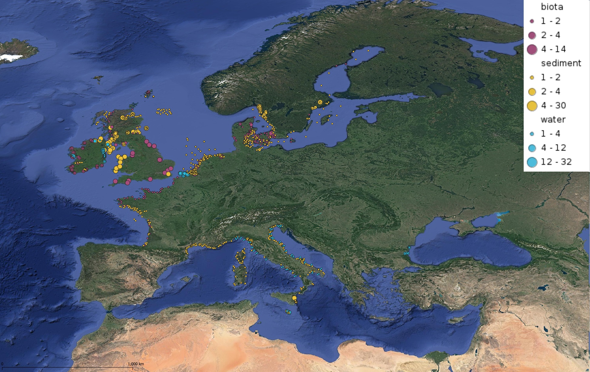
This product displays positions symbolized per matrix, for all available contaminants measurements for each year present in EMODnet regional contaminants aggregated datasets, v2022. The product displays positions for every available year.

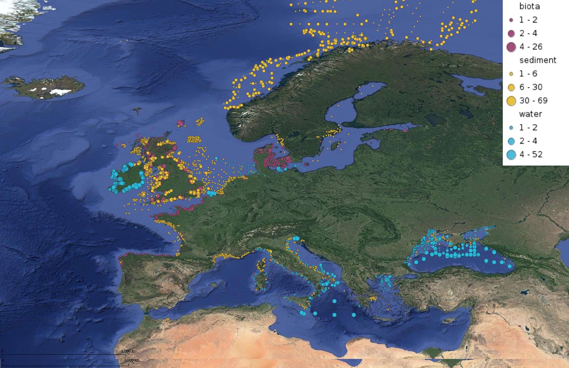
This product displays for Tributyltin, positions with values counts that have been measured per matrix for each year and are present in EMODnet regional contaminants aggregated datasets, v2022. The product displays positions for every available year.

This dataset comprises the global frequency, classification and distribution of marine heat waves (MHWs) from 1996-2020, in Chauhan et al. 2023 (https://doi.org/10.3389/fmars.2023.1177571). The classification was done based on their attributes and using different baselines. Daily SST values were extracted from the NOAA-OISST v2 high-resolution (0.25°) dataset from 1982-2020. MHWs were detected using the method presented by Hobday et al. 2016 (https://doi.org/10.1016/j.pocean.2015.12.014), and by using the 95th percentile of the accumulated temperature distribution to flag the extreme events. A shifting baseline of 8-year rolling period was selected between the years 1982-1996, since this period shows relatively stable maximum values of temperature across different ocean regions. The shifting baseline aims to account for the decadal changes of westerly winds, temperatures and ocean gyres circulations. The classification was done using the KMeans clustering algorithm to identify the relevant features of MHWs and classify them into separate groups based on feature similarities. This algorithm takes MHW features, namely duration, maximum intensity, rate onset and rate decline, as input vectors and applies clustering in the 4-dimensional feature space where each data point represents an MHW event. Note that all the MHWs features are standardized because unequal variances can put more weight on variables with smaller variances. This record comprehends the geospatial datasets of: Average number of MHW days per year (i.e., the sum of all MHW days divided by the total number of years, 1996-2020). Average cumulative intensity per year (i.e., the sum of cumulative intensity divided by the total number of years, 1996-2020). Total number of MHW events across the different periods averaged on the total number of years (1989-2020). The period 1982-1988 was only used as an initial baseline without calculating MHWs. Spatial distribution of three MHW categories: moderate MHWs, abrupt and Intense MHWs and extreme MHWs; displaying the total number of MHW days normalized by the number of years considered (i.e., 1989-2020). Distribution of Extreme MHWs across the different periods (A) 1989-1996, (B) 1997-2004, (C) 2005-2012, (D) 2013-2020. The relative frequency (γ) is a ratio of extreme MHWs in a specific period and all extreme MHWs in the same cluster for all periods.

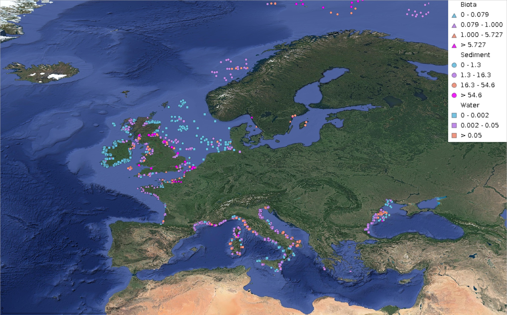
This product displays for Naphthalene, median values of the last 6 available years that have been measured per matrix and are present in EMODnet regional contaminants aggregated datasets, v2022. The median values ranges are derived from the following percentiles: 0-25%, 25-75%, 75-90%, >90%. Only "good data" are used, namely data with Quality Flag=1, 2, 6, Q (SeaDataNet Quality Flag schema). For water, only surface values are used (0-15 m), for sediment and biota data at all depths are used.

This product displays for Benzo(a)pyrene, positions with values counts that have been measured per matrix for each year and are present in EMODnet regional contaminants aggregated datasets, v2022. The product displays positions for every available year.