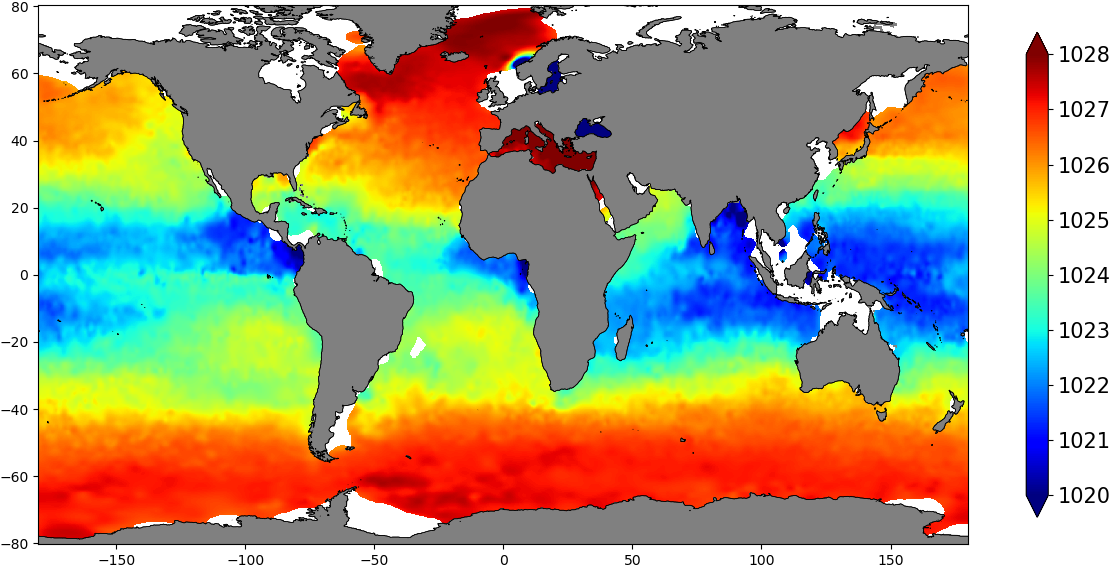
The SDC_GLO_CLIM_Dens product contains global monthly climatological estimates of in situ density using Temperature and Salinity from profiling floats contained in the World Ocean Data 18 (WOD18) database. The profiles were first quality controlled with a Nonlinear Quality control procedure. The climatology considers observations from surface to 2000 m for the time period 2003-2017. Density profiles are computed using UNESCO 1983 (EOS 80) equation from in situ temperature, salinity and pressure measurements by the PFL. Only profiles with both T,S values were used. The gridded fields are computed using DIVAnd (Data Interpolating Variational Analysis) version 2.3.1.

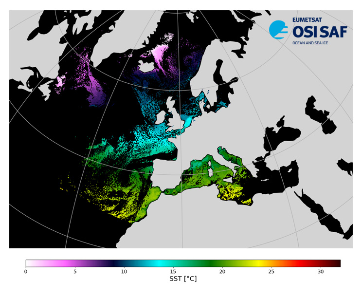
Level 3, four times a day, sub-skin Sea Surface Temperature derived from AVHRR on Metop satellites and VIIRS or AVHRR on NOAA and NPP satellites, over North Atlantic and European Seas and re-projected on a polar stereographic at 2 km resolution, in GHRSST compliant netCDF format. This catalogue entry presents NOAA-20 North Atlantic Regional Sea Surface Temperature. SST is retrieved from infrared channels using a multispectral algorithm and a cloud mask. Atmospheric profiles of water vapor and temperature from a numerical weather prediction model, Sea Surface Temperature from an analysis, together with a radiative transfer model, are used to correct the multispectral algorithm for regional and seasonal biases due to changing atmospheric conditions. The quality of the products is monitored regularly by daily comparison of the satellite estimates against buoy measurements. The product format is compliant with the GHRSST Data Specification (GDS) version 2.Users are advised to use data only with quality levels 3,4 and 5.

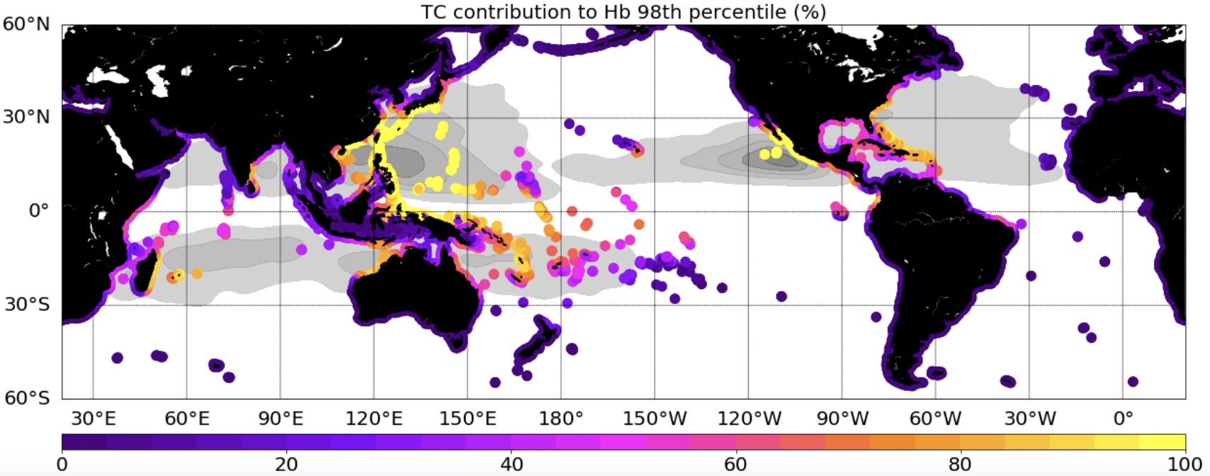
This dataset provides extreme waves (Hs: significant wave height, Hb:breaking wave height, a proxy of the wave energy flux) simulated with the WWIII model, and extracted along global coastlines. Two simulations, including or not Tropical Cyclones (TCs) in the forcing wind field, are provided.

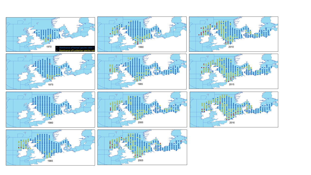
This metadata describes the ICES data on the temporal development of the Lusitanian/Boreal species ratio in the period from 19657 to 2016. Key message: The ratio between the number of Lusitanian (warm-favouring) and Boreal (cool-favouring) species are significantly increasing in several North-East Atlantic marine areas whereas there is no significant changes in all the southern areas. Changes in ratios are most apparent in the North Sea, Irish Sea and West of Scotland. Furthermore, it seems that Lusitanian species have not spread in all northward directions, but have followed two particular routes, through the English Channel and north around Scotland Blue dots indicates L/B ratios below 1 (dominance of Boreal species) Yellow dots indicates L/B ratios >=1 and <2 (dominance of Lusitanian species) Red dots indicates L/B ratios >=2 (high dominance of Lusitanian species) The dataset is derived from the ICES data portal 'DATRAS' (the Database of Trawl Surveys). DATRAS is an online database of trawl surveys with access to standard data products. DATRAS stores data collected primarily from bottom trawl fish surveys coordinated by ICES expert groups. The survey data are covering the Baltic Sea, Skagerrak, Kattegat, North Sea, English Channel, Celtic Sea, Irish Sea, Bay of Biscay and the eastern Atlantic from the Shetlands to Gibraltar. At present, there are more than 56 years of continuous time series data in DATRAS, and survey data are continuously updated by national institutions. The dataset has been used in the EEA Indicator "Changes in fish distribution in European seas" https://www.eea.europa.eu/data-and-maps/indicators/fish-distribution-shifts/assessment-1. The dataset has been used for this static map: https://www.eea.europa.eu/en/analysis/indicators/changes-in-fish-distribution-in/temporal-development-of-the-ratio

'''DEFINITION''' The CMEMS MEDSEA_OMI_tempsal_extreme_var_temp_mean_and_anomaly OMI indicator is based on the computation of the annual 99th percentile of Sea Surface Temperature (SST) from model data. Two different CMEMS products are used to compute the indicator: The Iberia-Biscay-Ireland Multi Year Product (MEDSEA_MULTIYEAR_PHY_006_004) and the Analysis product (MEDSEA_ANALYSISFORECAST_PHY_006_013). Two parameters have been considered for this OMI: * Map of the 99th mean percentile: It is obtained from the Multi Year Product, the annual 99th percentile is computed for each year of the product. The percentiles are temporally averaged over the whole period (1987-2019). * Anomaly of the 99th percentile in 2020: The 99th percentile of the year 2020 is computed from the Near Real Time product. The anomaly is obtained by subtracting the mean percentile from the 2020 percentile. This indicator is aimed at monitoring the extremes of sea surface temperature every year and at checking their variations in space. The use of percentiles instead of annual maxima, makes this extremes study less affected by individual data. This study of extreme variability was first applied to the sea level variable (Pérez Gómez et al 2016) and then extended to other essential variables, such as sea surface temperature and significant wave height (Pérez Gómez et al 2018 and Alvarez Fanjul et al., 2019). More details and a full scientific evaluation can be found in the CMEMS Ocean State report (Alvarez Fanjul et al., 2019). '''CONTEXT''' The Sea Surface Temperature is one of the Essential Ocean Variables, hence the monitoring of this variable is of key importance, since its variations can affect the ocean circulation, marine ecosystems, and ocean-atmosphere exchange processes. As the oceans continuously interact with the atmosphere, trends of sea surface temperature can also have an effect on the global climate. In recent decades (from mid ‘80s) the Mediterranean Sea showed a trend of increasing temperatures (Ducrocq et al., 2016), which has been observed also by means of the CMEMS SST_MED_SST_L4_REP_OBSERVATIONS_010_021 satellite product and reported in the following CMEMS OMI: MEDSEA_OMI_TEMPSAL_sst_area_averaged_anomalies and MEDSEA_OMI_TEMPSAL_sst_trend. The Mediterranean Sea is a semi-enclosed sea characterized by an annual average surface temperature which varies horizontally from ~14°C in the Northwestern part of the basin to ~23°C in the Southeastern areas. Large-scale temperature variations in the upper layers are mainly related to the heat exchange with the atmosphere and surrounding oceanic regions. The Mediterranean Sea annual 99th percentile presents a significant interannual and multidecadal variability with a significant increase starting from the 80’s as shown in Marbà et al. (2015) which is also in good agreement with the multidecadal change of the mean SST reported in Mariotti et al. (2012). Moreover the spatial variability of the SST 99th percentile shows large differences at regional scale (Darmariaki et al., 2019; Pastor et al. 2018). '''CMEMS KEY FINDINGS''' The Mediterranean mean Sea Surface Temperature 99th percentile evaluated in the period 1987-2019 (upper panel) presents highest values (~ 28-30 °C) in the eastern Mediterranean-Levantine basin and along the Tunisian coasts especially in the area of the Gulf of Gabes, while the lowest (~ 23–25 °C) are found in the Gulf of Lyon (a deep water formation area), in the Alboran Sea (affected by incoming Atlantic waters) and the eastern part of the Aegean Sea (an upwelling region). These results are in agreement with previous findings in Darmariaki et al. (2019) and Pastor et al. (2018) and are consistent with the ones presented in CMEMS OSR3 (Alvarez Fanjul et al., 2019) for the period 1993-2016. The 2020 Sea Surface Temperature 99th percentile anomaly map (bottom panel) shows a general positive pattern up to +3°C in the North-West Mediterranean area while colder anomalies are visible in the Gulf of Lion and North Aegean Sea . This Ocean Monitoring Indicator confirms the continuous warming of the SST and in particular it shows that the year 2020 is characterized by an overall increase of the extreme Sea Surface Temperature values in almost the whole domain with respect to the reference period. This finding can be probably affected by the different dataset used to evaluate this anomaly map: the 2020 Sea Surface Temperature 99th percentile derived from the Near Real Time Analysis product compared to the mean (1987-2019) Sea Surface Temperature 99th percentile evaluated from the Reanalysis product which, among the others, is characterized by different atmospheric forcing). Note: The key findings will be updated annually in November, in line with OMI evolutions. '''DOI (product):''' https://doi.org/10.48670/moi-00266

Le partenariat entre l’ensapBx et le GIP ATGeRi a permis la réalisation d’un atlas numérique via le catalogue et le visualiseur PIGMA. Cet atlas numérique donne accès à : - une carte sur laquelle sont situés des travaux d’étudiants et enseignants de l’ensapBx, - un lien vers le portail ArchiRès dans lequel sont décrits ces travaux de l’ensapBx avec téléchargement du document (lorsqu’il a été numérisé). De nombreux documents ont été référencés par l'ensapBx dans le catalogue PIGMA. Ils portent essentiellement sur les TPFE (travail personnel de fin d'études) et les PFE (projet de fin d'études). Ce référencement est alimenté progressivement par de nouveaux travaux.

The SDC_GLO_CLIM_N2 product contains seasonally averaged Brunt-Vaisala squared frequency profiles using the density profiles computed in SeadataCloud Global Ocean Climatology - Density Climatology. The Density Climatology product uses the Profiling Floats (PFL) data from World Ocean database 18 for the time period 2003 to 2017 with a Nonlinear Quality procedure applied on it. Computed BVF profiles are averaged seasonally into 5x5 degree boxes for Atlantic and Pacific Oceans. For data access, please register at http://www.marine-id.org/.

'''DEFINITION''' The Strong Wave Incidence index is proposed to quantify the variability of strong wave conditions in the Iberia-Biscay-Ireland regional seas. The anomaly of exceeding a threshold of Significant Wave Height is used to characterize the wave behavior. A sensitivity test of the threshold has been performed evaluating the differences using several ones (percentiles 75, 80, 85, 90, and 95). From this indicator, it has been chosen the 90th percentile as the most representative, coinciding with the state-of-the-art. Two Copernicus Marine products are used to compute the Strong Wave Incidence index: * IBI-WAV-MYP: '''IBI_MULTIYEAR_WAV_005_006''' * IBI-WAV-NRT: '''IBI_ANALYSISFORECAST_WAV_005_005''' The Strong Wave Incidence index (SWI) is defined as the difference between the climatic frequency of exceedance (Fclim) and the observational frequency of exceedance (Fobs) of the threshold defined by the 90th percentile (ThP90) of Significant Wave Height (SWH) computed on a monthly basis from hourly data of IBI-WAV-MYP product: SWI = Fobs(SWH > ThP90) – Fclim(SWH > ThP90) Since the Strong Wave Incidence index is defined as a difference of a climatic mean and an observed value, it can be considered an anomaly. Such index represents the percentage that the stormy conditions have occurred above/below the climatic average. Thus, positive/negative values indicate the percentage of hourly data that exceed the threshold above/below the climatic average, respectively. '''CONTEXT''' Ocean waves have a high relevance over the coastal ecosystems and human activities. Extreme wave events can entail severe impacts over human infrastructures and coastal dynamics. However, the incidence of severe (90th percentile) wave events also have valuable relevance affecting the development of human activities and coastal environments. The Strong Wave Incidence index based on the Copernicus Marine regional analysis and reanalysis product provides information on the frequency of severe wave events. The IBI-MFC covers the Europe’s Atlantic coast in a region bounded by the 26ºN and 56ºN parallels, and the 19ºW and 5ºE meridians. The western European coast is located at the end of the long fetch of the subpolar North Atlantic (Mørk et al., 2010), one of the world’s greatest wave generating regions (Folley, 2017). Several studies have analyzed changes of the ocean wave variability in the North Atlantic Ocean (Bacon and Carter, 1991; Kushnir et al., 1997; WASA Group, 1998; Bauer, 2001; Wang and Swail, 2004; Dupuis et al., 2006; Wolf and Woolf, 2006; Dodet et al., 2010; Young et al., 2011; Young and Ribal, 2019). The observed variability is composed of fluctuations ranging from the weather scale to the seasonal scale, together with long-term fluctuations on interannual to decadal scales associated with large-scale climate oscillations. Since the ocean surface state is mainly driven by wind stresses, part of this variability in Iberia-Biscay-Ireland region is connected to the North Atlantic Oscillation (NAO) index (Bacon and Carter, 1991; Hurrell, 1995; Bouws et al., 1996, Bauer, 2001; Woolf et al., 2002; Tsimplis et al., 2005; Gleeson et al., 2017). However, later studies have quantified the relationships between the wave climate and other atmospheric climate modes such as the East Atlantic pattern, the Arctic Oscillation pattern, the East Atlantic Western Russian pattern and the Scandinavian pattern (Izaguirre et al., 2011, Martínez-Asensio et al., 2016). The Strong Wave Incidence index provides information on incidence of stormy events in four monitoring regions in the IBI domain. The selected monitoring regions (Figure 1.A) are aimed to provide a summarized view of the diverse climatic conditions in the IBI regional domain: Wav1 region monitors the influence of stormy conditions in the West coast of Iberian Peninsula, Wav2 region is devoted to monitor the variability of stormy conditions in the Bay of Biscay, Wav3 region is focused in the northern half of IBI domain, this region is strongly affected by the storms transported by the subpolar front, and Wav4 is focused in the influence of marine storms in the North-East African Coast, the Gulf of Cadiz and Canary Islands. More details and a full scientific evaluation can be found in the CMEMS Ocean State report (Pascual et al., 2020). '''CMEMS KEY FINDINGS''' The trend analysis of the SWI index for the period 1980–2024 shows statistically significant trends (at the 99% confidence level) in wave incidence, with an increase of at least 0.05 percentage points per year in regions WAV1, WAV3, and WAV4. The analysis of the historical period, based on reanalysis data, highlights the major wave events recorded in each monitoring region. In region WAV1 (panel B), the maximum wave event occurred in February 2014, resulting in a 28% increase in strong wave conditions. In region WAV2 (panel C), two notable wave events were identified in November 2009 and February 2014, with increases of 16–18% in strong wave conditions. Similarly, in region WAV3 (panel D), a major event occurred in February 2014, marking one of the most intense events in the region with a 20% increase in storm wave conditions. Additionally, a comparable storm affected the region two months earlier, in December 2013. In region WAV4 (panel E), the most extreme event took place in January 1996, producing a 25% increase in strong wave conditions. Although each monitoring region is generally affected by independent wave events, the analysis reveals several historical events with above-average wave activity that propagated across multiple regions: November–December 2010 (WAV3 and WAV2), February 2014 (WAV1, WAV2, and WAV3), and February–March 2018 (WAV1 and WAV4). The analysis of the near-real-time (NRT) period (from January 2024 onward) identifies a significant event in February 2024 that impacted regions WAV1 and WAV4, resulting in increases of 20% and 15% in strong wave conditions, respectively. For region WAV4, this event represents the second most intense event recorded in the region. '''DOI (product):''' https://doi.org/10.48670/moi-00251

Maisons de la communauté

The technologies developed will expand our knowledge of the ocean’s interconnected systems and provide tangible benefits to the industries that rely on them, such as fisheries and aquaculture. The data generated will also support conservation initiatives and provide vital information to policy makers. The future impact of these valuable technologies relies on their accessibility. Therefore, TechOceanS technology pilots will be low-cost and place minimal demands on existing infrastructure, allowing them to be made available for use by all countries regardless of resources. TechOceanS will also work with the IOC-UNESCO to develop “ocean best practices” standards for training and monitoring of metrology and ocean systems.