 Catalogue PIGMA
2019
Type of resources
Available actions
Topics
Keywords
Contact for the resource
Provided by
Years
Formats
Representation types
Update frequencies
status
Service types
Scale
Resolution
-
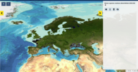
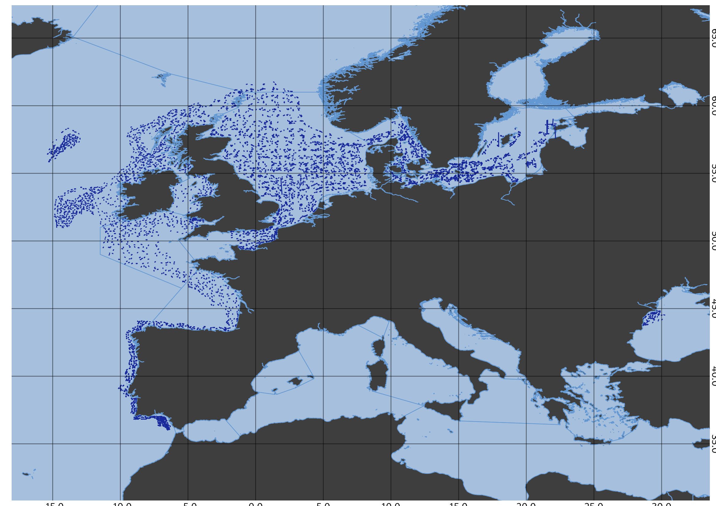
This product displays the stations present in EMODnet validated dataset where cadmium levels have been measured in water. EMODnet Chemistry has included the gathering of contaminants data since the beginning of the project in 2009. For the maps for EMODnet Chemistry Phase III, it was requested to plot data per matrix (water,sediment, biota), per biological entity and per chemical substance. The series of relevant map products have been developed according to the criteria D8C1 of the MSFD Directive, specifically focusing on the requirements under the new Commission Decision 2017/848 (17th May 2017). The Commission Decision points to relevant threshold values that are specified in the WFD, as well as relating how these contaminants should be expressed (units and matrix etc.) through the related Directives i.e. Priority substances for Water. EU EQS Directive does not fix any threshold values in sediments. On the contrary Regional Sea Conventions provide some of them, and these values have been taken into account for the development of the visualization products. To produce the maps the following process has been followed: 1. Data collection through SeaDataNet standards (CDI+ODV) 2. Harvesting, harmonization, validation and P01 code decomposition of data 3. SQL query on data sets from point 2 4. Production of map with each point representing at least one record that match the criteria The harmonization of all the data has been the most challenging task considering the heterogeneity of the data sources, sampling protocols. Preliminary processing were necessary to harmonize all the data : • For water: contaminants in the dissolved phase; • For sediment: data on total sediment (regardless of size class) or size class < 2000 μm • For biota: contaminant data will focus on molluscs, on fish (only in the muscle), and on crustaceans • Exclusion of data values equal to 0
-
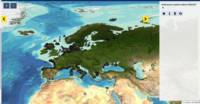
This product displays the stations present in EMODnet validated dataset where naphthalene levels have been measured in sediment. EMODnet Chemistry has included the gathering of contaminants data since the beginning of the project in 2009. For the maps for EMODnet Chemistry Phase III, it was requested to plot data per matrix (water,sediment, biota), per biological entity and per chemical substance. The series of relevant map products have been developed according to the criteria D8C1 of the MSFD Directive, specifically focusing on the requirements under the new Commission Decision 2017/848 (17th May 2017). The Commission Decision points to relevant threshold values that are specified in the WFD, as well as relating how these contaminants should be expressed (units and matrix etc.) through the related Directives i.e. Priority substances for Water. EU EQS Directive does not fix any threshold values in sediments. On the contrary Regional Sea Conventions provide some of them, and these values have been taken into account for the development of the visualization products. To produce the maps the following process has been followed: 1. Data collection through SeaDataNet standards (CDI+ODV) 2. Harvesting, harmonization, validation and P01 code decomposition of data 3. SQL query on data sets from point 2 4. Production of map with each point representing at least one record that match the criteria The harmonization of all the data has been the most challenging task considering the heterogeneity of the data sources, sampling protocols. Preliminary processing were necessary to harmonize all the data : • For water: contaminants in the dissolved phase; • For sediment: data on total sediment (regardless of size class) or size class < 2000 μm • For biota: contaminant data will focus on molluscs, on fish (only in the muscle), and on crustaceans • Exclusion of data values equal to 0
-
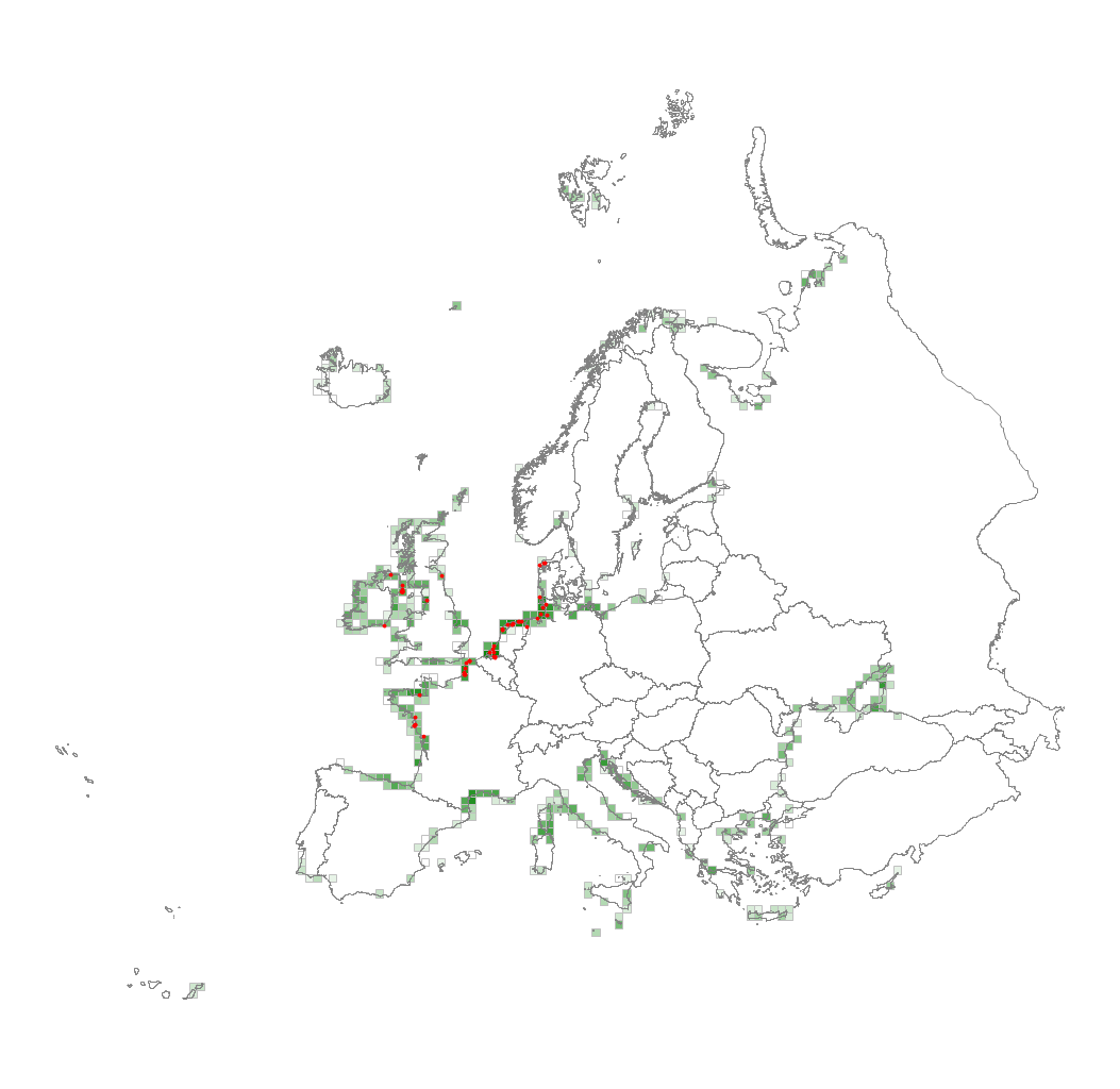
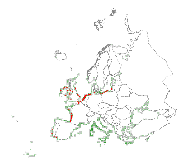
This metadata corresponds to the EUNIS Littoral biogenic habitat types (salt marshes), distribution based on vegetation plot data dataset. Littoral biogenic habitats (commonly known as salt marshes) are formed by animals such as worms and mussels or plants. The verified saltmarsh habitat samples used are derived from the Braun-Blanquet database (http://www.sci.muni.cz/botany/vegsci/braun_blanquet.php?lang=en) which is a centralised database of vegetation plots and comprises copies of national and regional databases using a unified taxonomic reference database. The geographic extent of the distribution data are all European countries except Armenia and Azerbaijan. The dataset is provided both in Geodatabase and Geopackage formats.
-
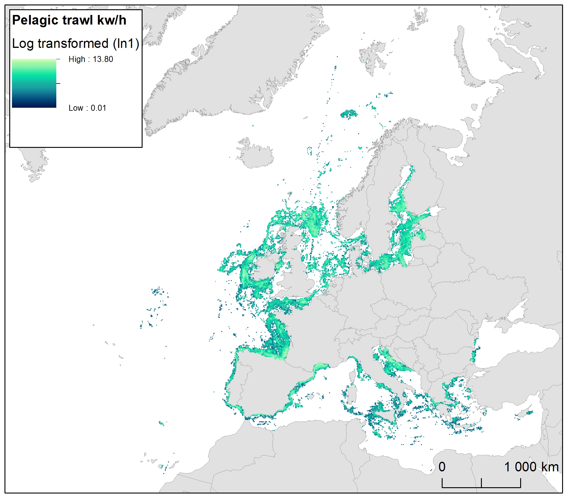
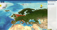
The raster dataset represents fishing intensity (kilowatt per fishing hour) by pelagic towed gears in the European seas. The dataset has been derived from Automatic Identification System (AIS) based pelagic fishing intensity data received from the European Commission’s Joint Research Centre - Independent experts of the Scientific, Technical and Economic Committee for Fisheries (JRC STECF), as well as from Vessel Monitoring System (VMS) and logbook based pelagic fishing effort data from HELCOM Commission. The temporal extent varies between the data sources (between 2013 and 2015). The dataset has been transformed to a logarithmic scale (ln1). This dataset has been prepared for the calculation of the combined effect index, produced for the ETC/ICM Report 4/2019 "Multiple pressures and their combined effects in Europe's seas" available on: https://www.eionet.europa.eu/etcs/etc-icm/etc-icm-report-4-2019-multiple-pressures-and-their-combined-effects-in-europes-seas-1.
-
This product displays the stations where benzo[A]pyrene has been measured and the values present in EMODnet Chemistry infrastructure are either above or below the limit of detection or quantification (LOD/LOQ), i.e for the substance, in that station, quality values found in EMODnet validated dataset can be equal to 6, Q or 1. It is necessary to take into account that LOD/LOQ can change with time. These products aggregate data by station, producing only one final value for each station (above, below or above/below). EMODnet Chemistry has included the gathering of contaminants data since the beginning of the project in 2009. For the maps for EMODnet Chemistry Phase III, it was requested to plot data per matrix (water,sediment, biota), per biological entity and per chemical substance. The series of relevant map products have been developed according to the criteria D8C1 of the MSFD Directive, specifically focusing on the requirements under the new Commission Decision 2017/848 (17th May 2017). The Commission Decision points to relevant threshold values that are specified in the WFD, as well as relating how these contaminants should be expressed (units and matrix etc.) through the related Directives i.e. Priority substances for Water. EU EQS Directive does not fix any threshold values in sediments. On the contrary Regional Sea Conventions provide some of them, and these values have been taken into account for the development of the visualization products. To produce the maps the following process has been followed: 1. Data collection through SeaDataNet standards (CDI+ODV) 2. Harvesting, harmonization, validation and P01 code decomposition of data 3. SQL query on data sets from point 2 4. Production of map with each point representing at least one record that match the criteria The harmonization of all the data has been the most challenging task considering the heterogeneity of the data sources, sampling protocols. Preliminary processing were necessary to harmonize all the data : • For water: contaminants in the dissolved phase; • For sediment: data on total sediment (regardless of size class) or size class < 2000 μm • For biota: contaminant data will focus on molluscs, on fish (only in the muscle), and on crustaceans • Exclusion of data values equal to 0
-
This product displays the stations where anthracene has been measured and the values present in EMODnet Chemistry infrastructure are always above the limit of detection or quantification (LOD/LOQ), i.e quality value equal to 1. It is necessary to take into account that LOD/LOQ can change with time. These products aggregate data by station, producing only one final value for each station (above, below or above/below). EMODnet Chemistry has included the gathering of contaminants data since the beginning of the project in 2009. For the maps for EMODnet Chemistry Phase III, it was requested to plot data per matrix (water,sediment, biota), per biological entity and per chemical substance. The series of relevant map products have been developed according to the criteria D8C1 of the MSFD Directive, specifically focusing on the requirements under the new Commission Decision 2017/848 (17th May 2017). The Commission Decision points to relevant threshold values that are specified in the WFD, as well as relating how these contaminants should be expressed (units and matrix etc.) through the related Directives i.e. Priority substances for Water. EU EQS Directive does not fix any threshold values in sediments. On the contrary Regional Sea Conventions provide some of them, and these values have been taken into account for the development of the visualization products. To produce the maps the following process has been followed: 1. Data collection through SeaDataNet standards (CDI+ODV) 2. Harvesting, harmonization, validation and P01 code decomposition of data 3. SQL query on data sets from point 2 4. Production of map with each point representing at least one record that match the criteria The harmonization of all the data has been the most challenging task considering the heterogeneity of the data sources, sampling protocols. Preliminary processing were necessary to harmonize all the data : • For water: contaminants in the dissolved phase; • For sediment: data on total sediment (regardless of size class) or size class < 2000 μm • For biota: contaminant data will focus on molluscs, on fish (only in the muscle), and on crustaceans • Exclusion of data values equal to 0
-
This product displays the stations present in EMODnet validated dataset where cadmium levels have been measured in sediment. EMODnet Chemistry has included the gathering of contaminants data since the beginning of the project in 2009. For the maps for EMODnet Chemistry Phase III, it was requested to plot data per matrix (water,sediment, biota), per biological entity and per chemical substance. The series of relevant map products have been developed according to the criteria D8C1 of the MSFD Directive, specifically focusing on the requirements under the new Commission Decision 2017/848 (17th May 2017). The Commission Decision points to relevant threshold values that are specified in the WFD, as well as relating how these contaminants should be expressed (units and matrix etc.) through the related Directives i.e. Priority substances for Water. EU EQS Directive does not fix any threshold values in sediments. On the contrary Regional Sea Conventions provide some of them, and these values have been taken into account for the development of the visualization products. To produce the maps the following process has been followed: 1. Data collection through SeaDataNet standards (CDI+ODV) 2. Harvesting, harmonization, validation and P01 code decomposition of data 3. SQL query on data sets from point 2 4. Production of map with each point representing at least one record that match the criteria The harmonization of all the data has been the most challenging task considering the heterogeneity of the data sources, sampling protocols. Preliminary processing were necessary to harmonize all the data : • For water: contaminants in the dissolved phase; • For sediment: data on total sediment (regardless of size class) or size class < 2000 μm • For biota: contaminant data will focus on molluscs, on fish (only in the muscle), and on crustaceans • Exclusion of data values equal to 0
-
This metadata corresponds to the EUNIS Coastal habitat types, distribution based on vegetation plot data dataset. Coastal habitats are those above spring high tide limit (or above mean water level in non-tidal waters) occupying coastal features and characterised by their proximity to the sea, including coastal dunes and wooded coastal dunes, beaches and cliffs. Includes free-draining supralittoral habitats adjacent to marine habitats which are normally only very rarely subject to any type of salt water, in as much as they may be inhabited predominantly by terrestrial species, strandlines characterised by terrestrial invertebrates and moist and wet coastal dune slacks and dune-slack pools. Supralittoral sands and wracks may be found also in marine habitats (M). Excludes supralittoral rock pools and habitats, the splash zone immediately above the the mean water line, as well the spray zone and zone subject to sporadic inundation with salt water in as much as it may be inhabited predominantly by marine species, which are included in marine (M). The verified coastal habitat samples used are derived from the Braun-Blanquet database (http://www.sci.muni.cz/botany/vegsci/braun_blanquet.php?lang=en) which is a centralised database of vegetation plots and comprises copies of national and regional databases using a unified taxonomic reference database. The geographic extent of the distribution data are all European countries except Armenia and Azerbaijan. The dataset is provided both in Geodatabase and Geopackage formats.
-
EMODnet Chemistry aims to provide access to marine chemistry data sets and derived data products concerning eutrophication, ocean acidification, contaminants and litter. The chosen parameters are relevant for the Marine Strategy Framework Directive (MSFD), in particular for descriptors 5, 8, 9 and 10. The datasets contain standardized, harmonized and validated data collections from seafloor litter. Datasets concerning seafloor litter data are loaded in a central database after a semi-automated validation phase. Once loaded, a data assessment is performed in order to check data consistency and potential errors are corrected thanks to a feedback loop with data originators. EMODnet seafloor litter data and database are hosted and maintained by ‘Istituto Nazionale di Oceanografia e di Geofisica Sperimentale, Division of Oceanography (OGS/NODC)’ from Italy. For seafloor litter, the harmonized datasets contain all unrestricted EMODnet Chemistry data on seafloor litter data, including 12438 CDI records. The temporal range covered is from 2006-10-01 to 2018-08-16. Data are formatted following Guidelines and forms for gathering marine litter data, which can be found at: https://doi.org/10.6092/15c0d34c-a01a-4091-91ac-7c4f561ab508. The harmonized datasets can be downloaded as EMODnet Sea-floor litter data format Version 1.0, which is a csv file, tab separated values. The original datasets can be searched and downloaded from EMODnet Chemistry Download Service: https://emodnet-chemistry.maris.nl/search
-
This product displays the stations present in EMODnet validated dataset where benzo[A]pyrene levels have been measured in biota. EMODnet Chemistry has included the gathering of contaminants data since the beginning of the project in 2009. For the maps for EMODnet Chemistry Phase III, it was requested to plot data per matrix (water,sediment, biota), per biological entity and per chemical substance. The series of relevant map products have been developed according to the criteria D8C1 of the MSFD Directive, specifically focusing on the requirements under the new Commission Decision 2017/848 (17th May 2017). The Commission Decision points to relevant threshold values that are specified in the WFD, as well as relating how these contaminants should be expressed (units and matrix etc.) through the related Directives i.e. Priority substances for Water. EU EQS Directive does not fix any threshold values in sediments. On the contrary Regional Sea Conventions provide some of them, and these values have been taken into account for the development of the visualization products. To produce the maps the following process has been followed: 1. Data collection through SeaDataNet standards (CDI+ODV) 2. Harvesting, harmonization, validation and P01 code decomposition of data 3. SQL query on data sets from point 2 4. Production of map with each point representing at least one record that match the criteria The harmonization of all the data has been the most challenging task considering the heterogeneity of the data sources, sampling protocols. Preliminary processing were necessary to harmonize all the data : • For water: contaminants in the dissolved phase; • For sediment: data on total sediment (regardless of size class) or size class < 2000 μm • For biota: contaminant data will focus on molluscs, on fish (only in the muscle), and on crustaceans • Exclusion of data values equal to 0